Output from the TramoSeats procedure
The TRAMO-SEATS method consists of two linked programs: TRAMO and SEATS. The results from TRAMO are displayed in the Output from a modelling procedure section. This section focuses on the nodes that arenot described there, in particular on the output produced by SEATS. Therefore, the sections that are explained here are: Main results, Decomposition, Benchmarking and Diagnostics. Their content is accessible once the user selects the appropriate node from the left-hand side seasonal adjustment results panel.
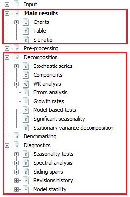
The structure of the results for TRAMO-SEATS
Main results
On the very top of the Main results window, vital messages related to the seasonal adjustment process are displayed (if any). They should be examined by the user as they indicate potential issues with the seasonal adjustment process that hinder the decomposition or even make it impossible. Some illustrative examples are given below.
When the time series is shorter than 3 years JDemetra+ is not able to perform the decomposition due to an insufficient number of observations.
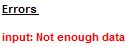
Error message displayed because of not enough available observations
Although the procedure can be executed in the presence of outliers and missing values, their particular composition can stop the decomposition procedure. This is the case when missing values or outliers cumulate in a specific period (e.g. the data gap is observed each year in March) and therefore the results from the TRAMO model are not reliable enough to perform the decomposition.
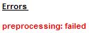
Error message due to a concentration of missing values in a particular period
In both cases discussed above the time series cannot be estimated neither by the TRAMO nor by RegARIMA.
When the model chosen by TRAMO is further changed by SEATS, JDemetra+ displays the following warning.
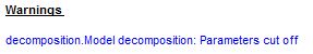
Information about the change of the ARIMA model made by SEATS
Further sections of the Main results node includes summary information from TRAMO and SEATS and presents the main statistics that assess the quality of the outcomes.
Information about the TRAMO part of the process includes the estimation span, number of observations, transformation (if any) and deterministic effects. This is discussed in detail in the Model summary section.
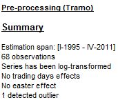
The summary of the results from TRAMO
In the case of the pre-defined specifications RSA0, RSA1 and RSA3 no trading day effect is estimated. For the RSA2 and RSA4 pre-defined specifications, working day effects and the leap year effect are pre-tested and estimated if present. If the working day effect is significant, the pre-processing part includes the message Working days effect (1 regressor). The message Working days effect (2 regressors) means that both the working day effect and the leap year effect were estimated. For RSA5 and RSAfull the trading day effect and the leap year effect are pre-tested. If the trading day effect has been detected, either of the messages Trading days effect (6 regressors) or Trading days effect (7 regressors) are displayed, depending whether the leap year effect were detected or not. If the Easter effect is statistically significant, the message Easter effect detected is displayed.
The second part of the Main results panel presents the innovation variances of the orthogonal1 components estimated by SEATS, which result from the decomposition of a stochastic time series (i.e. the original series corrected for the deterministic effects and missing observations). These components are trend, seasonal, transitory and irregular and derive from the decomposition of the stochastic (linearized) time series \(x_{t}\). In the case of an additive decomposition, \(x_{t}\ \)can be presented as a sum of the components:
| \[x_{t} = \sum_{i = 1}^{k}x_{\text{it}}\] | [1] |
where:
\(i\) – trend, seasonal, transitory or irregular components, respectively.
The linearised series \(x_{t}\ \)follows an ARIMA model of the type:
| \[\phi(B)\delta\left( B \right)x_{t} = \theta(B)a_{t}\] | [2] |
where:
\(\delta\left( B \right)\) – a non-stationary autoregressive (AR) polynomial in \(B\) (unit roots);
\(\theta\left( B \right)\) – an invertible moving average (MA) polynomial in \(B\), which is a product of the invertible regular MA polynomial in \(B\) and the invertible seasonal MA polynomial in \(B^{S}\).2
\(\phi(B)\) – a stationary autoregressive (AR) polynomial in \(B\) and a stationary seasonal polynomial in\(\ B^{S}\).
\(a_{t}\) – a white-noise variable with the variance\(\ V(a)\), also referred as innovation.3
Each component follows the general ARIMA model3:
\({\phi_{i}\left( B \right)\delta}_{i}\left( B \right)\ x_{\text{it}} = \theta_{i}(B)a_{\text{it}}\) [3]
where:
\(a_{\text{it}}\sim WN(0,V\left( a_{i} \right))\) is an i. i. d. white-noise innovation of the\(\ i^{\text{th}}\) component; it is also an estimator of the 1-period-ahead forecast error of the\(\ i^{\text{th}}\) component.
The polynomials\(\ \theta_{i}(B)\), \(\phi_{i}(B)\) and \(\delta_{i}\left( B \right)\) are of finite order. A white-noise variable is normally, identically and independently distributed, with a zero-mean and variance of the component innovation (the variance of the 1-period ahead forecast error of the component) \(V\left( a_{i} \right)\). Two different components do not share the same unit autoregressive roots.
The components can be also expressed in a compact form:
| \(\varphi_{i}\left( B \right)x_{\text{it}} = \theta_{i}(B)a_{\text{it}}\), | [4] |
where \(\varphi_{i}\left( B \right)\) is a product of the stationary (\(\delta_{i}\left( B \right))\ \)and the non-stationary (\(\phi_{i}(B))\ \)autoregressive polynomials.
SEATS decomposition fulfils the canonical property, i.e. it maximizes the variance of the irregular component providing trend, seasonal and transitory components as stable as possible (in accordance with the models)4. For each component the value of the innovation variance \(k_{i}\ \)is represented by the ratio of the component innovation variance \(V\left( a_{i} \right)\) to the variance of the series innovation \(V\left( a \right)\):5
| \(k_{i} = \frac{V(a_{i})}{V(a)}\). | [5] |
The innovations in the components are the cause of their stochastic behaviour (i.e., their moving features). The larger the variance, the more volatile the component will be6. In general, interest centres on more stable seasonal signals and hence when competing models are compared, the preferred one is the model that minimizes the innovation variance of the seasonal and trend components7. Such solution results in the trend and the seasonal component that are as smooth and stable as possible, and the irregular component that absorb as much noise as possible.
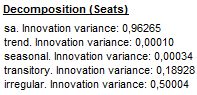
The summary of the results from SEATS
The Diagnostics section is displayed below the summary of the decomposition results produced by SEATS. It includes the outcome of the most important quality indicators. They are discussed in the Diagnostics section. The results are accompanied by two figures. The one on the left shows the original series, the final seasonally adjusted series, and the final trend.
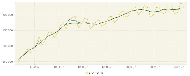
The original series and the results from decomposition: the seasonally adjusted series and the trend.
The local menu, which can be activated by right clicking on the graph, contains the following options:
-
Select all – selects all time series presented in the graph;
-
Show title – this option is not currently available;
-
Show legend – displays titles of all time series presented on the graph;
-
Edit format – enables the user to change data format;
-
Color scheme – allows the user to change the colour in the graph;
-
Lines thickness – allows the user to choose between thin and thick lines to be used for a graph;
-
Show all – this option is not currently available;
-
Export RM_C_pic to – allows the graph to be sent to the printer and saved to the clipboard or as a file in PNG format;
-
Configure – enables the user to customize chart and series display.
The panel on the right shows the SI ratios.
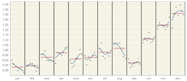
The SI ratios
The Main results three subsections: Charts, Table and S-I ratio node provide visual presentation of the decomposition results. The Charts section includes two graphs. The first one shows the original series, trend and seasonally adjusted series together with the forecasts for the next year for each of these series.
The original series, trend and the seasonally adjusted series together with the forecasts
The second graph from the Charts section presents the calendar effects, the seasonal component and the irregular component. As a rule, the calendar component is expected to be weaker than the seasonal component; however it is not the case for a non-seasonal series with calendar effects present. The irregular component is assumed to be random and unpredictable; therefore its forecasts are, in general, zero (for the additive model) or one (for the multiplicative model). The lack of certain movements (seasonal and/or irregular) is manifested by a horizontal line with values equal to zero (for the additive model) or one (for the multiplicative model).
The decomposition results: calendar effects, the seasonal component and the irregular component. Seas (component) stands for the seasonal component
For both charts the local menu, which is activated by right click on the graph, offers the same set of options as the ones available for the chart presented below Figure The original series and the results from decomposition above. The Table section presents the data for the original series with forecasts, the final seasonally adjusted series, the trend with forecasts, the seasonal component with forecasts and the irregular component. In general, the irregular component, by definition, cannot be forecast, therefore for TRAMO-SEATS its forecasts are set to 0 (additive model) or 1 (multiplicative model). However, there are some exceptions from this rule. Firstly, when the transitory component has been extracted, it is not displayed in a separate table, but together with the irregular component. In such case the forecasts displayed in the Irregular column result from forecasting of the transitory component. Secondly, non-zero irregular forecasts can also be explained by the presence of TC outliers (especially when they were identified at the end of the series), as these outliers generate the effect that decays in time8. Finally, in the case of log models, SEATS performs a bias correction to ensure that the irregular and seasonal components are, on average, equal to 1. The correction factor is also applied to the forecasts, which are then not exactly 1 (but they are constant). When the X-13ARIMA-SEATS method is used no values for the forecasting period of the irregular component are computed, following the approach implemented in the original software.
The local menu, activated by right clicking on the table, contains the same functions that are available for Grid. All series are extended with one year of forecasts. These forecasts are presented in the bottom part of the table.
Decomposition results presented as a table
The S-I ratio chart presents the seasonal-irregular (S-I) component and the seasonal factors for each of the periods in the time series (months or quarters). The seasonal-irregular component is calculated as the ratio of the original series to the estimated trend, thus it presents an estimate of the detrended series. Blue curves represent the final seasonal factors and the red straight lines represent the mean seasonal factor for each period.
S-I ratios
Decomposition
SEATS receives the linearised series from TRAMO. The decomposition made by SEATS assumes that all components in time series – trend, seasonal, transitory (if present) and irregular – are orthogonal and can be expressed by the ARIMA model. SEATS performs the canonical decomposition of the components, which assumes that only irregular components include noise. Each model is presented in a closed form (i.e. using the backshift operator \(B\)). In the main page of the Decomposition node the following items are presented (if estimated):
-
Model – the ARIMA model for the linearised series and the innovation variance of the model for the linearised series;
-
Sa – the ARIMA model for the seasonally adjusted series and the innovation variance of the model for the seasonally adjusted series;
-
Trend – the ARIMA model for the trend component of the series and the innovation variance of the model for the trend;
-
Seasonal – the ARIMA model for the seasonal component of the series and the innovation variance of the model for the seasonal component;
-
Transitory – the ARIMA model for the transitory component of the series and the innovation variance of the model for the transitory component;
-
Irregular – The innovation variance of the irregular component.
The trend component captures the low-frequency variation of the series and displays a spectral peak at a frequency 0. By contrast, the seasonal component picks up the spectral peaks at seasonal frequencies and the irregular component captures a white noise process. The transitory component, which is the additional component estimated by SEATS for some time series, can be seen as a noise-free, detrended and seasonally adjusted time series. This component captures a highly transitory variation that is not a white noise and should not be assigned neither to the seasonal component nor the trend component. It also captures spectral peaks at frequencies that are neither zero nor seasonal9. The model for the transitory component is a stationary ARMA model, with low-order MA components (order \(Q - P\), when \(Q > P\))10 and AR roots with small moduli that should not be included neither in the trend component nor in the seasonal component.
The example of the time series decomposition calculated by SEATS is presented below. It can be seen that the overall autoregressive polynomial has been factorized into the polynomials assigned to the components according to the frequencies of the roots. As an example, the model for the trend is: ARIMA(1,2,3)(0,0,0) with an innovation variance 0.22517.
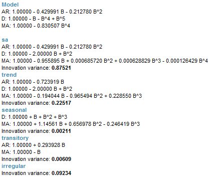
The ARIMA models for original series, seasonally adjusted series and components
The decomposition above is performed for the ARIMA model identified by TRAMO. However, in some cases, the ARIMA model chosen by TRAMO is changed by SEATS11. It is done, for example, when the ARIMA model selected by TRAMO leads to a non-admissible decomposition. In this case, the ARIMA model chosen by SEATS is displayed in the Pre-processing → Arima section of the result panel and this model is used to decompose the series.
In the Pre-processing → Arima section two spectra are presented: one from the TRAMO model and one from the SEATS model.
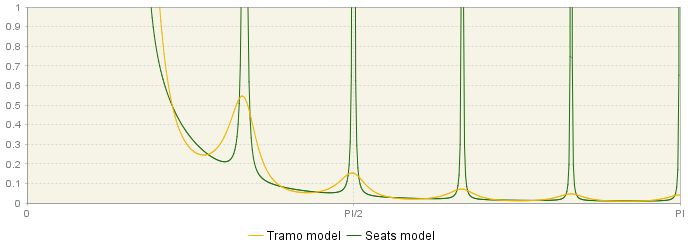
Theoretical spectrum of the ARIMA model
Under the section where the polynomials and the regular AR roots from the TRAMO model are reported, the respective information is also displayed for the model identified by SEATS.
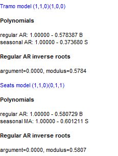
Comparison of the two ARIMA model used for modelling – the TRAMO model and the SEATS model
Stochastic series
A discrete-time stochastic process is a collection of random variables ${ X_{t}(\omega)}$, where \(t\) denotes time and \(\omega\) denotes an elementary event. A time series associated with these random variables is called a stochastic time series. In general, a stochastic time series is made of two components, one which is predictable once the history of the process \(X_{t - 1}\) is known, and one that is not.
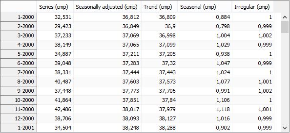
This part of the output presents the results of the decomposition of the stochastic series resulting from the linearisation procedure performed by TRAMO. The main panel incorporates the table containing the following series produced by SEATS:
-
Series (lin);
-
Seasonally adjusted (lin);
-
Trend (lin);
-
Seasonal (lin);
-
Irregular (lin);
-
Seasonally adjusted (stde lin);
-
Trend (stde lin);
-
Seasonal (stde lin);
-
Irregular (stde lin) (contains transitory component, if any).
Lin is an abbreviation from linearised series (including a logarithmic transformation of the data if the multiplicative decomposition is used) and stde denotes standard deviation. All series are extended with one year of forecasts. These forecasts are presented in the bottom part of the table.
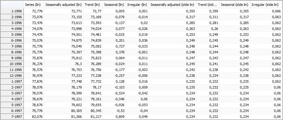
Stochastic series extended with forecasts
The two subsections allow for some insights into the development of the two components (trend and seasonal) in the last 7 years and a forecast for the next year. For each component its values are displayed with the associated 95% confidence intervals, highlighting the fact that these values result from the estimation procedure. The width of the confidence intervals shows the size of uncertainty of the estimation results, which, in general, is greater at the end of the time series. The prediction intervals, which are available for the forecasts, are even wider than the confidence intervals. The graph is available for the trend and for the seasonal component, as illustrated on the figures below, respectively.
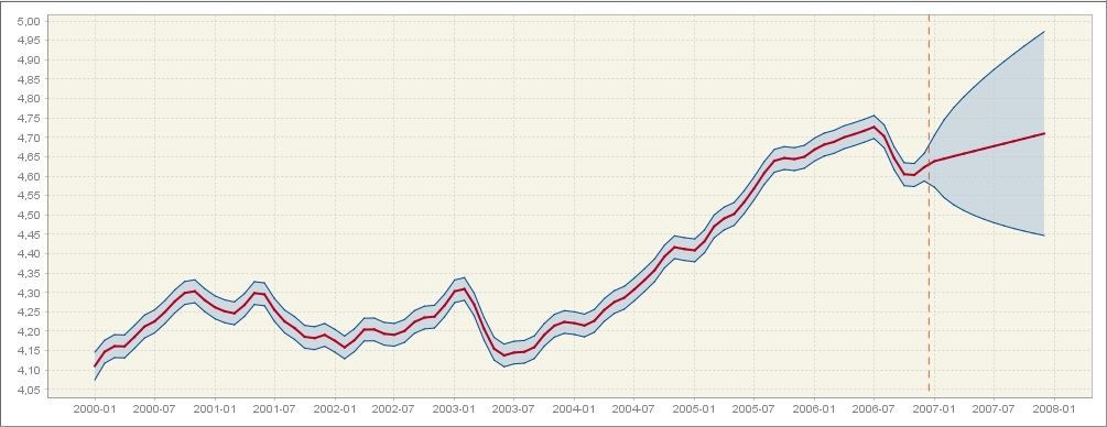
The trend estimate with the confidence interval and the prediction interval
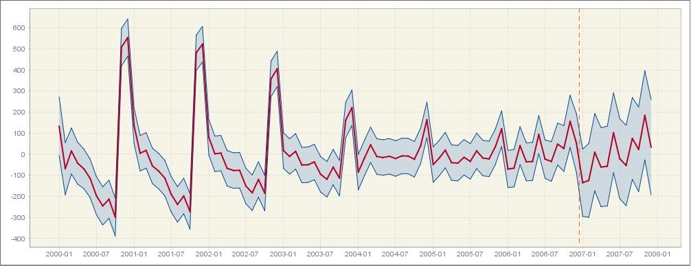
The seasonal component estimate with the confidence interval and the prediction interval
Components
The Components section presents the values of the components estimated from the ARIMA model applied to the linearised series. Cmp is an abbreviation from component.
The theoretical components calculated from the ARIMA model applied to the linearized series
WK analysis – Components
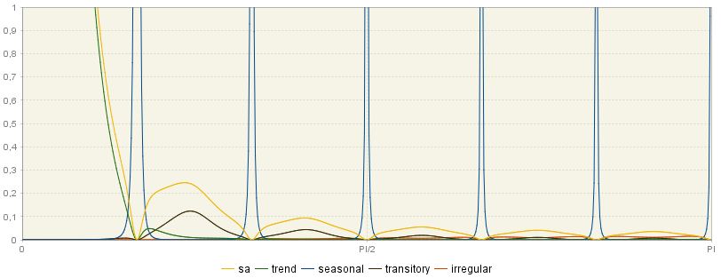
This section presents the (pseudo) spectra of the components and seasonally adjusted series calculated from the ARIMA models presented in the main panel of the Decomposition section. The sum of the spectra of the components should be equal to the spectrum of the linearised time series, which is presented in the Pre-processing → Arima node. When the TRAMO model has not been accepted by SEATS, the spectra of the components derive from the ARIMA model changed by SEATS. The spectrum of the seasonally adjusted series (yellow) is the sum of the spectra of the trend component (green), the transitory component, if present (black), and the irregular component (orange).
The stochastic variability in the \(i^{\text{th}}\) component is generated by the innovations \(a_{\text{it}}\). Therefore, small values of variance innovations \(V\left( a_{i} \right)\) are associated with a stable component, and large values of \(V\left( a_{i} \right)\) with an unstable component. The spectrum of the \(i^{\text{th}}\) component is proportional to \(V\left( a_{i} \right)\). Further, stable trend and seasonal components are those with thin spectral peaks, while unstable ones are characterised by wide spectral peaks.
If a series contains an important component for a certain frequency, its spectrum should reveal a peak around that frequency. As a trend can be thought as a cyclical component with an infinite length of the movement, the spectral peak should occur at the frequency \(\omega = 0\).12 For a monthly time series there are six seasonal frequencies: \(\frac{\pi}{6}\), \(\frac{2\pi}{6},\ \frac{3\pi}{6},\ \frac{4\pi}{6},\frac{5\pi}{6},\pi\), while for a quarterly data there are two seasonal frequencies: \(\ \frac{\pi}{2},\pi\). The spectrum for a seasonal component has peaks around these frequencies.
In the figure below the standard spectra for trend (green), seasonal (blue), transitory (black) and irregular (orange) are displayed. As it was already explained, the frequency \(\omega = 0\) is associated with a trend. For the frequencies in the range [\(0 + \epsilon_{1},\ \frac{\pi}{2} - \epsilon_{2}\)] with \(\epsilon_{1},\ \epsilon_{2} > 0\) and \(\epsilon_{1} < \ \frac{\pi}{2} - \epsilon_{2}\ \)the associated period will be longer than a year and bounded13. The frequencies in the range [\(\frac{\pi}{2},\ \pi\)] are associated with short term movements, with a cycle completed in less than a year. Finally, the peak in the transitory component is an evidence of a trading day effect.
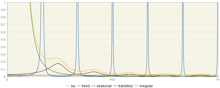
The theoretical spectra of the components and the seasonally adjusted series
The ACGF (stationary) window displays the pseudo-autocovariance generating functions14 of the stationary components. They are theoretical values (i.e. they are not computed on the linearised series, but on the ARIMA model).
ACGF function of the stationary components
WK analysis – Final estimators
The various graphs that can be found in this section show the results of the estimation of the components performed with the Wiener-Kolmogorov (WK) filters15. The Wiener-Kolmogorov filters are symmetric and bi-infinite, which requires that for each observation included in the filter the past and future observations exist. Obviously, they are not available for the observations in the beginning and at the end of the time series. In order to apply a filter to all observations from \(x_{t}\), the original, linearised time series is extended with forecasts and backcasts using an ARIMA model, which has been chosen in the TRAMO phase of seasonal adjustment. Then, SEATS applies the filter to the extended series16. As a new observation (i.e. observation for the period\(\ t + 1\)) is available, the forecast for the period \(t + 1\) is replaced by this new observation and all forecasts for the periods \(g > t + 1\) are updated. It means that at the end of the time series the estimator of the component is preliminary and is subject to revisions, while in the central periods the estimator can be treated as a final one (also called a historical estimator)17.
Regarding the importance of final (historical) estimators, which are derived by applying the WK filters, JDemetra+ presents several graphs showing their properties (see Wiener-Kolmogorow filter section in SEATS) the corresponding graphs for the components and for the final estimators of the components vary, as components and final estimators follow different models. For example, the seasonal component follows the model:\(\ \phi_{s}\left( B \right)s_{t} = \theta_{s}(B)a_{t}\), while the corresponding MMSE estimator of the seasonal component follows the model: \(\phi_{s}\left( B \right){\widehat{s}}_{t} = \theta_{s}\left( B \right)\alpha_{s}(F)a_{t}\), where \(\alpha_{s}(F)\) is a difference between the theoretical component and the estimator.18
These graphs are listed below. For each graph all series from the graph can be copied (the Copy all visible). The graph can be saved and/or printed. These options are available from the local menu, which is available by right clicking on the graph.
Spectrum
The spectra17 of the final estimators are shown in the first graph. The spectrum of the estimator of the seasonal component is obtained by multiplying the squared gain19 of the filter by the spectrum of the linearised series.
From the example below it is clear that these spectra are similar to those of the components, although estimator spectra show spectral zeros at the frequencies where the component spectra are close but not exactly zero. The estimator adapts to the structure of the analysed series, i.e. the width of the spectral holes in the seasonally adjusted series (yellow line) depends on the width of the seasonal peaks in the seasonal component estimator spectrum (blue lines).4
Spectra of the final estimators
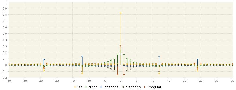
Square gain of components filter
The squared gain controls the extent to which a movement of particular amplitude at a frequency \(\omega\) is delivered to the output series. It determines how the variance of the series contributes to the variance of the component for the different frequencies. In other words, it specifies which frequencies will contribute to the signal (that is, it filters the spectrum of the series by frequencies).20 When the squared gain is zero in band \(\lbrack\omega_{1},\ \omega_{2}\rbrack\) it means that the output series is free of movements in this range of frequencies.21 On the contrary, when for some \(\omega\) the squared gain is 1, then all variation is passed on to the component estimator.
The figure below shows that the seasonal frequencies are assigned to the seasonal component while the seasonally adjusted series captures the non-seasonal frequencies. As a consequence, it is expected that the seasonal component estimator captures only the seasonal frequencies, so the square gain is close to 1 at seasonal frequencies. By contrast, the estimator of the non-seasonal part of the time series is expected to eliminate seasonal frequencies, leaving unmodified non-seasonal frequencies. Therefore, the squared gain of seasonally adjusted data should be nearly zero for seasonal frequencies.
The squared gain shape depends on the model used for the time series. The two figures below show squared gains derived from two different models are represented. In the first figure, the squared gain of the seasonal adjustment filter shows relatively large troughs to suppress a highly stochastic seasonal component. In contrast, the second figure presents the estimators for a seasonal component, which is much more deterministic than the previous one.
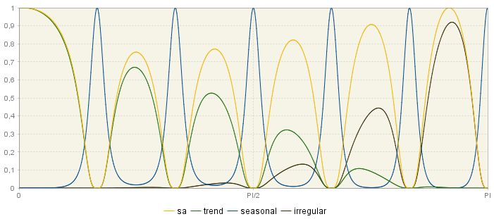
Squared gains for filters of component series – the case of a stochastic seasonal component
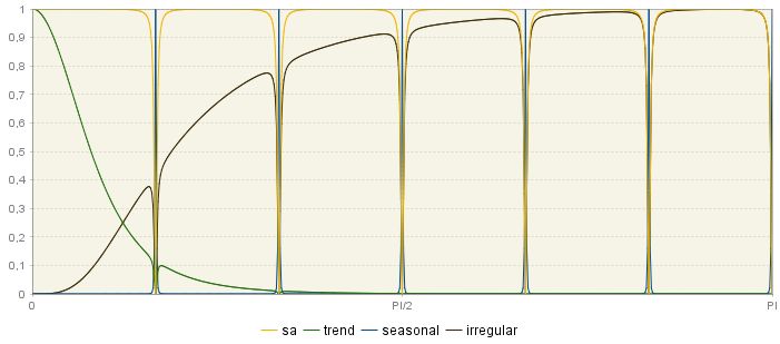
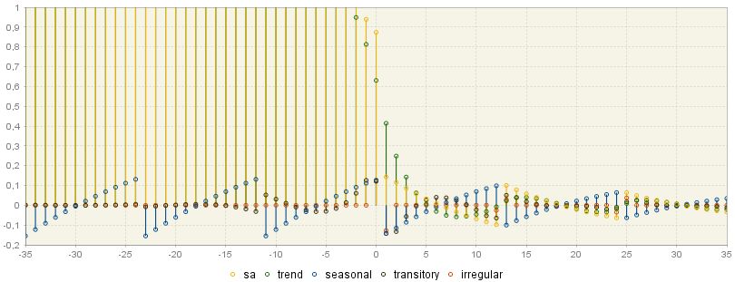
Squared gains for filters of component series – the case of a deterministic seasonal component
WK filters
The Wiener-Kolmogorov (WK) filter \(\nu_{i}(B,F)\) shows the weights that have been applied to the original series \(x_{t}\ \)to estimate the \(\ {\widehat{x}}_{\text{it}}\ \)component in the following way (see Wiener-Kolmogorow filter section in SEATS for a description of the WK filter):
\(\widehat{x}_{\text{it}} = \nu_{i}\left( B,F \right)x_{t}\) [6]
where:
| \(\nu_{i}\left( B,F \right) = \nu_{0} + \sum_{j = 0}^{\infty}{(B^{j} + F^{j}})\) | [7] |
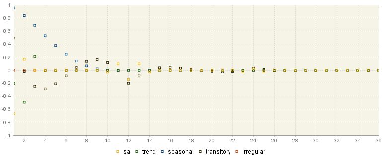
Since each WK filter is symmetric and centred, it is also convergent, which enables the user to approximate an infinite number of realizations \(x_{t}\) by a finite number of terms (from the graph below it could be noticed that\(\ j = 36\), so the WK filter includes \(36 + 1 + 36 = 73\) terms).
Since WK filters are symmetric, centered and convergent, they are valid for computing the estimators in the central periods of the sample. The following graph demonstrates the weights that are applied to each observation for each component to calculate the estimate of each component.
WK filter weights for the seasonally adjusted series and for the components
The highest weights are applied to the central observations and the weights decrease for observations further away in time. The weighting pattern depends on the component. For example, in the case of the seasonal component the greatest weights are applied to the current value and the past and future values from this same period. On the contrary, the estimate of the trend at a given point in time is mostly influenced by the current value and few preceding and following values of the linearised series.
PsiE-weights
PsiE-weights (\(\psi\)) are a different representation of the final estimator, i.e. this representation shows the estimator as a filter applied to the innovations \(\text{ a}_{t}\), rather than the series \(\text{ x}_{t}\)22. The figure below shows for each component how the contribution of the total innovation to the component estimator \(\widehat{x}_{\text{it}}\) varies in time (the size of this contribution is shown on the Y-axis). For the non-negative values on the X-axis, PsiE-weights show the effect of starting conditions, present and past innovations in series, while for negative observations they present the effect of future innovations. It can be seen that they are non-convergent in the past (they are convergent when series \(\text{ x}_{t}\) is stationary). On the contrary, the effect of future innovations is a zero-mean and convergent process. PsiE-weights are important to analyse the convergence of estimators and revision errors.
PsiE-weights for the components
Error analysis
Being obtained by using forecasts, the component estimators at the end points of the series are preliminary and are subject to revisions as future data become available, until it can be assumed that the final (historical) estimator has been reached. This process typically last between 3 and 5 years. The error analysis deals with the size of error variances and speed of their convergence to the final value.
From the model-based structure it is possible to determine the underlying models for the two types of errors: revision error and estimation error. Thus the respective variances, autocorrelations and spectra can be computed. The speed of convergence of the revision can also be assessed. For each \(i^{\text{th}}\) component, the total error in the preliminary estimator \(d_{it|t + k}\) is expressed as:
\(d_{it|t + k} = x_{\text{it}} - {\widehat{x}}_{it|t + k}\) [8]
where:
\(x_{\text{it}}\) is the \(i^{\text{th}}\ \)component;
\(\widehat{x}_{it|t + k}\) is the estimator of \(x_{\text{it}}\) when the last observation is \(x_{t + k}\) ($x_{t}$ is a time series).
The total error in the preliminary estimator can be also presented as a sum of the final estimation error (\(e_{\text{it}}\)) and the revision error (\(r_{it|t + k}\)), i.e.:
\(d_{it|t + k} = x_{\text{it}} - {\widehat{x}}_{it|t + k} = \left( x_{\text{it}} - {\widehat{x}}_{\text{it}} \right) + \left( {\widehat{x}}_{\text{it}} - {\widehat{x}}_{it|t + k} \right) = e_{\text{it}} + r_{it|t + k}\) [9]
The final estimation error (\(e_{\text{it}}\)) and the revision error (\(r_{it|t + k}\)) are orthogonal23.
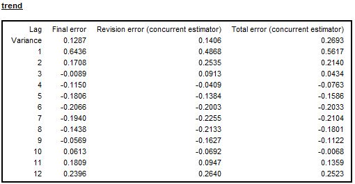
The errors analysis (variance and ACF of the total error and its components) is available for the trend and for the seasonally adjusted series. The values are given in units of variance of the innovations in the linearized series. Therefore, from the examples presented below it can be noticed that the variance of the concurrent estimator of the seasonally adjusted series is roughly 17% of the variance of the innovations of the linearized series and 27% for the trend (see the two figures below, respectively).
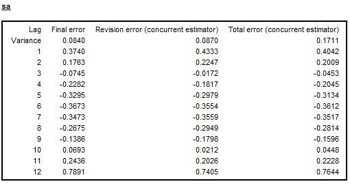
Autocorrelation of the errors for the seasonally adjusted series – the case of deterministic seasonal pattern
Autocorrelation of the errors for the trend – the case of a non-seasonal series
As stressed by MARAVALL, A. (1995), large revisions are associated with highly stochastic components and converge quickly, while smaller revisions are implied by very stable components and converge slowly. In general, the slow convergence of the SA series estimator to the final estimator suggests that very little would be gained from moving from a current adjustment to a concurrent one24. When several models for a given series are compared, the preferred model is the one for which the historical estimation error is minimal and convergence of revision errors is relatively fast, even if the resulting ARIMA model is optimal from the TRAMO perspective.
The last table available in the Errors analysis panel presents the convergence of a concurrent estimator measured by the revision error, which is the difference between a preliminary estimator and a final estimator. For each component the table shows the percentage reduction in the standard error of the revision after an additional year (up to 5 years). Comparisons are made with the concurrent estimators. This table informs about the time needed by the concurrent estimators to converge to the final ones and therefore how many periods it takes for a new observation to no longer significantly affect the estimate.
For the series used to produce Figure 5.41, Figure 5.42 and Figure 5.43 the estimated innovation variance of the seasonal component is 0.02135 which implies that this component is fairly stable, while the trend component, for which the innovation variance is 0.11526, is more stochastic. The convergence of the SA series is slow (Figure 5.43), so in this case the current adjustment strategy would imply a little loss in precision of the SA series. It is because the stable component is of little importance in explaining the series variability; therefore the removal of this component implies a small revision error, which tends to converge slowly25.
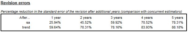
Revision errors analysis up to five years of observations
When a series is non-seasonal and a non-seasonal ARIMA model is used, then the autocorrelation errors table for seasonally adjusted data is not displayed. In this case the final error, the revision error and the total error, displayed for the trend component, converge to zero swiftly.

Autocorrelation of the errors for the trend component – the case of a non-seasonal series
Growth rates
The tables in this section show, starting with a concurrent estimation, the convergence of the trend and seasonally adjusted series to their final estimators as new observations become available. The calculation is performed for the growth rates of the time series \(z_{t}\ \)over the period \((t - m,\ t)\). The error variances displayed in this section are based on the estimation error of the stochastic trend and the seasonally adjusted series. The errors in the parameter estimates are not considered.
When the multiplicative model is applied, the growth rate over the \(\text{m }\)periods is defined as \(\left( \frac{Z_{t}}{Z_{t_{t - m}}} - 1 \right) \times 100\). All standard errors reported for the growth rates in the following tables are computed using a linear approximation to the rates. When period-to-period changes are large, these standard errors should be interpreted as broad approximations, that will tend to underestimate the true values. In the case of the additive model the growth rate is given by the difference between \(z_{t_{t - m}}\) and \(z_{t}\).
The total estimation error is the largest for the first period (concurrent estimator) and it decreases (for preliminary estimators) until it reaches a constant value. This constant value is the standard deviation of the historic estimator. In the figure below the total estimation error for historic estimator is around 0.38. From the observation of convergence, it can be judged that after 6 periods a new observation no longer significantly affects the estimate (the standard error is 0.38% from this point onwards).
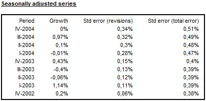
Analysis of growth rates for seasonally adjusted series
For the series presented in the figure above, the figure below illustrates that the trend estimator converges faster than that of the seasonally adjusted series because the trend component is stochastic while the seasonal component is rather stable.25 After 2 years (8 additional observations) all estimators have practically converged (revision error is close to zero).
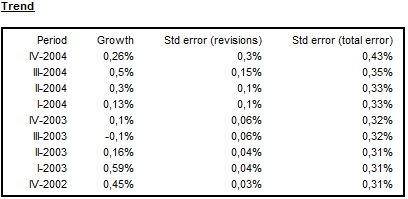
Analysis of growth rates for the trend
Model based tests
The Model-based tests section concentrates on the distribution of components, theoretical estimators and empirical estimates (stationary transformation). This node is divided into three sections.
Variance
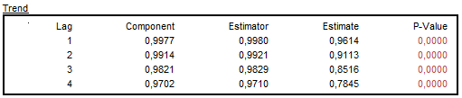
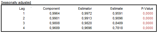
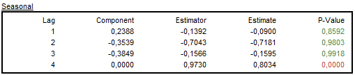
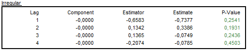
In this panel the variances of the component innovations are displayed (variance of the component innovation26, (Component), theoretical variances of the stationary transformation of the estimated components and empirical variances of the stationary transformation of the estimated components (Estimate)) are displayed25 (see also Main results section).
SEATS identifies the components assuming that, except for the irregular component, they are clean of noise. It implies that the variance of the irregular is maximized in contrast to the trend and seasonal components, which are as stable as possible. In this section JDemetra+ presents a table, which compares the variance of the stationary transformation of the innovations of the components (Component) with the variance of their theoretical estimators (Estimator) and the variance of their empirical (actually obtained) estimates (Estimate).
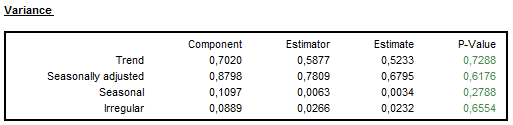
Variance of the components, their theoretical estimators and their empirical estimates (stationary transformation)
It follows from the properties of the MMSE (Minimum Mean Square Error) estimator that it will always underestimate the component (estimators always have a smaller variance than the components). The size of underestimation depends on the particular model. The underestimation is relatively large when the variance of the component is relatively small. It means that, for example, the trend estimator always has a smaller variance than the trend component and the ratio of the two variances increases as the trend becomes more stable. Therefore, the more stochastic the trend is, the closer the estimator variance is to the component variance. On the other hand, the variance of the estimator of a very stable trend will be considerably lower than the variance of the component27. It means that the trend estimator provides a more stable trend than the one implied by the theoretical model28.
For all components it is expected that29 the variance of the component innovation is greater than the variance of its theoretical estimators30. The later should be relatively close to the variance of the empirical estimate31. As a rule, if the correct WK filter was applied then the empirical variance will be in close agreement with the theoretical ones25. If for a given component, the variance of its theoretical estimators is significantly greater than the variance of its empirical estimate, then this component is underestimated. The opposite relationship indicates the overestimation of the component.
The outcome of the over/under estimation test is provided as a p-value in the last column of the table presented in the figure above. A p-value in green denotes that the problematic characteristic has not been detected. An outcome in yellow signals the uncertain results. An outcome in red implies that an issue should be addressed. For example, when for a given component, the variance of its theoretical estimator is significantly greater than the variance of its empirical estimate, this component is underestimated. Therefore, a p-value in red manifests a strong underestimation of the component variance; a p-value in yellow is a sign of a mild underestimation of the component variance; and a p-value in green indicates no underestimation of the component variance. On the contrary, if the variance of the theoretical estimator of a component is significantly lower than the variance of its empirical estimate, this indicates than this component is underestimated. In such case a p-value in red is interpreted as a strong overestimation of the component variance; a p-value in yellow indicate a mild overestimation of the component variance; and a p-value in green indicate no overestimation of the component variance.
Autocorrelation functions
The autocorrelation function (ACF)32 is a basic tool for time domain analysis of a time series. For each component and for the seasonally adjusted series, JDemetra+ exhibits autocorrelations of the stationary transformation of the components, the estimators and the sample estimates. They are calculated from the first regular lag up to the first seasonal lag. If the model is correct, the empirical estimate of the autocorrelation function should be close to the theoretical estimator of the autocorrelation function. However, for small values of the innovation variance\(\ \)the discrepancy between the ACF function of the components and of the estimator may be substantial. In general, the more stable a component is, the larger is the discrepancy28.
For each table displayed in the Autocorrelation section the p-values of the test are given in the last column. The user should check whether the empirical estimates agree with the model, i.e. if their ACF functions are close to those of the model for the estimators. Special attention should be given to the first and/or seasonal order autocorrelation23.
Meaning of the p-value for autocorrelation tests.
| Value | Colour | Meaning |
|---|---|---|
| Good | Green | no evidence of autocorrelation |
| Uncertain | Orange | mild evidence of autocorrelation |
| Bad | Red | strong evidence of autocorrelation |
It should be noted that this test does not provide information about the direction of the autocorrelation.
A comparison of the theoretical MMSE estimators with the estimates actually calculated can be used as a diagnostic tool for the model validation. The closeness of the estimators and estimates points towards validation of the results3. The failure of this test indicates the misspecification of the component models, which is often due to the replacement of a non-admissible TRAMO model with its decomposable approximation performed by SEATS1.
Examples of the ACF function for the components are presented below.
Autocorrelations of the stationary transformation of the trend, the estimators and the sample estimates
Autocorrelations of the stationary transformation of the seasonally adjusted series, the estimators and the sample estimates
Autocorrelations of the stationary transformation of the seasonal component, the estimators and the sample estimates
When the transitory component is not estimated, then the coefficients of the autocorrelation function of the irregular component are always zero (the Component column) as a theoretical model for the irregular component (\(u_{t}\)) is a white noise2. However the irregular estimator follows the ARMA model:
\(\widehat{u}_{t} = k_{u}\frac{1}{\psi(B)\psi(F)}x_{t}\) [10]
where \(k_{u} = \frac{Var(u)}{Var(a)}\).
The estimator \({\widehat{u}}_{t}\ \)is expressed as a linear function of present and future innovations. Therefore, it is autocorrelated (the Estimator column contains non-zero values).
When the transitory exists, the irregular and transitory component are estimated together. Therefore, in such situations the coefficients of the autocorrelation function of the irregular component might be non-zero (the Component column).
Autocorrelations of the stationary transformation of the irregular component, the estimators and the sample estimates
Cross-correlation function
The decomposition made by SEATS assumes orthogonal components. To test this assumption, JDemetra+ presents a table that contains cross-correlations between the stationary transformations of the components, the estimators and the actual estimates (theoretical components are uncorrelated). The cross-correlations are given for: trend and seasonal, trend and irregular, seasonal and irregular and, if the transitory is present, trend and transitory, seasonal and transitory, irregular and transitory.
Although components of the time series are assumed to be uncorrelated, their estimators can be correlated as the estimator variance will always underestimate the component variance. MMSE estimator implies a correlation between the estimators of the components3. For this reason a correlations between the stationary transformations of the estimators and of the estimates actually obtained should be checked3.
The first column gives the theoretical correlations. The second column provides the empirical correlation between the stationary transformations of the estimated components. Finally, the last column tests with the Bartlett’s approximations4 if the estimated correlations differ from their theoretical values.
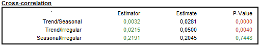
Correlation between the component estimators and the component sample estimates
It is expected that the theoretical cross-correlations between the component estimators will be close to their sample estimates5.
Significant seasonality
In a model-based seasonal adjustment the mean \(\widehat{s}_{i}\) and the variance \(\widehat{v}_{i}\) of the different components can be computed. Under the usual hypothesis of normal distributions, a straightforward way tests is applied to test if an estimate is significantly different from 0. This is done by comparing \(| \frac{\widehat{s}_{i}}{\sqrt{\widehat{v}_{i}}}|\) with the suited critical value.
The table displayed in this section presents the number of periods in one year where the seasonal component is significantly different from 0. As the standard deviations are time-varying, the test is performed at the middle of the series (historical), for the last year (current) and for the first year of forecasts.
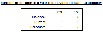
Number of periods in a year with a significant seasonality
Stationary variance decomposition
This section presents the relative contribution of components to the variance of the detrended original series.6 This decomposition reveals how the particular components contribute to the overall variance of the detrended series. This decomposition mirrors Table F2F of the original X-11 and it is based on the similar in LADIRAY, D., and QUENNEVILLE, B. (1999). Therefore, it can be used for a comparison of the results from both methods.
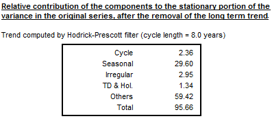
Relative contribution of the components to the stationary portion of the variance in the original series with the long term trend subtracted
Benchmarking
In the context of seasonal adjustment, benchmarking means the procedure that ensures the consistency over the calendar year between adjusted and non-seasonally adjusted data. It should be noted that the ‘ESS Guidelines on Seasonal Adjustment’ (2015) do not recommend benchmarking, as it introduces a bias in the seasonally adjusted data. Therefore, for the pre-defined specifications this option is disabled and in the results tree the Benchmarking node is empty. To activate it, click on the Specifications button, and then activate the checkbox Is enabled in the Benchmarking section and click Apply.
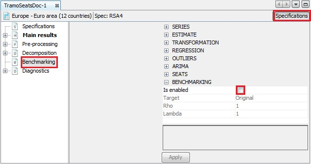
The Benchmarking option – a default view
The benchmaring procedure explained in the Benchmarking section.
Diagnostics
The Diagnostic panel contains detailed information on the quality of the seasonal adjustment. These diagnostics are divided into six sections: Matrix, Seasonality tests, Spectral analysis, Sliding spans, Revisions history and Model stability.
Main panel
The summary of the quality assessment is presented directly in the main panel of the Diagnostics node and is divided into several groups.
A range of indicators (tests) that measure the quality of seasonal adjustment results is offered by JDemetra+. This set is not identical with the sets implemented in the original seasonal adjustment programs. The interpretation of the outcomes of the tests could be problematic for an inexperienced user. For this reason, the outcomes of the tests are accompanied with the values of the qualitative indicator, which facilitate the assessment of the results from the process. The values of this qualitative indicator are given in the table below.
The values of the qualitative indicator.
| Value | Meaning |
|---|---|
| Undefined | The quality is undefined because of an unprocessed test, a meaningless test, a failure in the computation of the test, etc. |
| Error | There is a logical error in the results (for instance, it contains aberrant values or some numerical constraints are not fulfilled). The processing should be rejected. |
| Severe | There is no logical error in the results but they should not be accepted for serious quality reasons. |
| Bad | The quality of the results is bad following a specific criterion, but there is no actual error and the results can be used. |
| Uncertain | The result of the test shows that the quality of the seasonal adjustment is uncertain. |
| Good | The result of the test is good from the aspect of the quality of seasonal adjustment. |
Several qualitative indicators can be combined following the basic, arbitrary rules. In particular, it is done for the Summary indicator, which gives the first insight into the quality of the estimation and can be especially useful for the assessment of the seasonal adjustment of large datasets performed under time pressure. The quality assessment provided by the Summary indicator aims to support the user when the high number of series that are being treated makes it hard or even impossible to perform an individual analysis of the results, although an additional validation of the results by the user is recommended.

The value of the summary indicator for a given series
The rule for the calculation of the Summary indicator as well as other aggregated indicators, which combine \(n\) qualitative indicators, is given in the table below. To calculate the average of the (defined) diagnostics, 0 is assigned to Bad, 2 is assigned to Uncertain and 3 is assigned to Good.
The overall value of the aggregated indicator.
| Sum | Rules |
|---|---|
| Undefined | All of \(n\) qualitative indicators are Undefined. |
| Error | The value of at least one of \(n\) qualitative indicators is Error. |
| Severe | None of the \(n\) qualitative indicators is Error and at least one of them is Severe. |
| Bad | None of the \(n\) qualitative indicators is Error or Severe. The average of the (defined) diagnostics is less than 1.5. |
| Uncertain | None of the \(n\) qualitative indicators is Error or Severe. The average of the (defined) diagnostics is in the range [1.5, 2.5]. |
| Good | None of the \(n\) qualitative indicators is Error or Severe. The average of the (defined) diagnostics is at least 2.5. |
According to the table above, the Error and Severe diagnostics are unacceptable results.
The basic checks section includes two quality diagnostics: definition and annual totals.
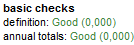
Basic checks tests results
The definition test inspects some basic relationships between different components of the time series. In the case of an additive decomposition the following relationships are checked:
-
mhe = ee + omhe
-
cal = tde + mhe
-
out = out_t + out_s + out_i
-
reg = reg_t + reg_s + reg_i + reg_y
-
reg_sa = reg_t + reg_i
-
det = cal + out + reg
-
c_t = t + o_t + reg_t
-
c_s = s + cal + o_s + reg_s
-
c_i = i + o_i + reg_i
-
c_sa = y_c − c_s = c_t + c_i + reg_y
-
cy_c = c_t + c_s + reg_y = t + s + i + reg
-
y_l = y_c − det = t + s + i
-
sa = y − s = t + i
-
si = y_l − t = s + i
The explanations of the abbreviation used in these formulas are given in the table below.
The components and effects used in the definition test formulas.
| Name | Definition |
|---|---|
| y | Original series |
| y_c | Interpolated time series (i.e.original time series with missing values replaced by their estimates) |
| t | Trend (without regression effect) |
| s | Seasonal (without regression effect) |
| i | Irregular (without regression effect) |
| sa | Seasonally adjusted series (without regression effect) |
| si | S-I ratio |
| tde | Trading day (or working day) effect |
| mhe | Moving holidays effect |
| ee | The Easter effect |
| omhe | Other moving holidays effect |
| cal | Calendar effects |
| out | Total outlier effect |
| out_t | Effect of outliers assigned to the trend component (LS) |
| out_s | Effect of outliers assigned to the seasonal component (SO) |
| out_i | Effect of outliers assigned to the irregular component (AO, TC) |
| reg | Effect of regression variables (except for outliers) |
| reg_t | Effect of regression variables (except for outliers) assigned to the trend component |
| reg_s | Effect of regression variables (except for outliers) assigned to the seasonal component |
| reg_i | Effect of regression variables (except for outliers) assigned to the irregular component |
| reg_y | Separate regression effects (except for outliers) |
| reg_sa | Effect of regression variables (except for outliers) assigned to the seasonally adjusted series |
| det | Deterministic effect |
| c_t | Trend, including deterministic effect |
| c_i | The irregular component, including deterministic effect |
| c_s | The seasonal component, including deterministic effect |
| c_y | The orginal series, including deterministic effect |
| c_sa | The seasonally adjusted series, including deterministic effect |
| cal_y | Calendar adjusted series |
| y_l | Linearized series |
A multiplicative model7 is obtained in the same way by replacing the operations “+” and “-“ by “*” and “/” respectively. The explanations of the abbreviations are given in the Output items section.
The definition test verifies that all the definition constraints are well respected. The maximum of the absolute differences is computed for the different equations and related to the Euclidean norm of the initial series (\(Q\)).
The threshold values for the results of the definition test.
| Q | Diagnostic |
|---|---|
| > 0.000001 | Error |
| <= 0.000001 | Good |
The annual totals test compares the annual totals of the original series with those of the seasonally adjusted series. The maximum of their absolute differences is computed and related to the Euclidean norm of the initial series.
The threshold values for the results of the annual totals test.
| **Q ** | Diagnostic |
|---|---|
| > 0.5 | Error |
| [0.1, 0.5] | Severe |
| [0.05, 0.1] | Bad |
| [0.01, 0.05] | Uncertain |
| <=0.01 | Good |
Several tests are computed on the residuals of the TRAMO model. The definition of the residuals slightly differs from those of the original X-13ARIMA-SEATS and the TRAMO-SEATS algorithms. However, their global messages are nearly always very similar.
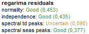
Tests on residuals from the RegARIMA model
The normality test (which combines skewness and kurtosis tests), displayed in the figure above, is the Doornik-Hansen test, which follows a\(\ \chi^{2}\) distribution.
The threshold values for the results of the Doornik-Hansen normality test.
| Pr( >val) | JDemetra+ default settings |
|---|---|
| <0.01 | Bad |
| [0.01, 0.1] | Uncertain |
| ≥0.1 | Good |
The independence test is the Ljung-Box test, which follows a \(\chi_{(k - np)\ }^{2}\) distribution, where \(k\) depends on the frequency of the series (24 for a monthly series, 8 for a quarterly series, \(4 \times freq\ \)for the other frequencies, where \(\text{freq}\) is a frequency of the time series) and \(\text{np}\) is the number of hyper-parameters of the model (number of parameters in the ARIMA model).
The threshold values for the results of the Ljung-Box test.
| Pr(>val) | JDemetra+ default settings |
|---|---|
| <0.01 | Bad |
| [0.01, 0.1] | Uncertain |
| ≥0.1 | Good |
JDemetra+ checks for the presence of trading day (spectral td peaks) and seasonal peaks (spectral seas peaks) in the residuals using a test based on the periodogram of the residuals. The periodogram is computed at the so-called Fourier frequencies. Under the hypothesis of a Gaussian white noise of the residuals, it is possible to derive a simple test on the periodogram, around specific (groups of) frequencies. The exact definition of the test is described here.
The threshold values for the results of the test on periodogram.
| P(stat>val) | JDemetra+ default settings |
|---|---|
| <0.001 | Severe |
| [0.001, 0.01] | Bad |
| [0.01, 0.1] | Uncertain |
| ≥0.1 | Good |
In the outliers section the result of the test that checks the number of outliers in relation to the series lengths is displayed. By default, the result of the test is acceptable if the relative number of outliers is below 3%. In general, a high number of outliers may indicate the problems with the model specification. However, in some cases the high share of the outliers in the series span is justified, e.g. when the series is affected by several methodological changes. The settings for this test can be modified in the Tools \(\mathbf{\rightarrow}\ \)Options menu, Demetra \(\mathbf{\rightarrow}\ \) Statistics section (see Tools in the Options section).
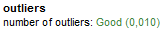
Test on outliers
Indicators in the SEATS section check if the crucial assumptions concerning the relationship between the components are fulfilled. These tests are discussed in the Model-based tests section above.
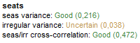
The summary results from decomposition performed by SEATS
Under the Summary indicator a set of tests that check for the presence of the residual seasonality is displayed. The residual seasonality diagnostics implemented in JDemetra+ correspond to the set of tests developed for X-12-ARIMA. One of them is the F-test for the presence of residual seasonality, which is computed on the detrended seasonally adjusted series and on the irregular component.
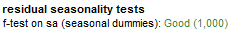
Residuals seasonality tests
In order to remove the trend from a monthly time series, a first order difference of lag three is applied (a first order difference of lag one in the other cases)33 to the seasonally adjusted series. For the detrended seasonally adjusted series the presence of residual seasonality is tested on the complete time span and on the last 3 years span. See here for the description of the test.
The threshold values for the results of the F-test for the presence of residual seasonality.
| P-value | JDemetra+ default settings |
|---|---|
| <0.01 | Severe |
| [0.01, 0.05] | Bad |
| [0.05, 0.1] | Uncertain |
| ≥0.1 | Good |
The F-test is also performed on a seasonally adjusted series to check if there is a significant trading days effect.
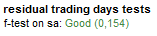
The result from the residual trading days test
Matrix
The Matrix node compares the results from the seasonal adjustment produced for the time series using all pre-defined and user-defined specifications. The list of all specifications is given in the first column. The one, which was chosen by the user to perform a seasonal adjustment is marked with [C]. The specifications’ names shown here correspond to the names used in the Workspace window. The results are divided into six tabs:
-
Main – main information on the ARIMA model:
-
N – number of observations;
-
Seasonal – a result of seasonality tests (1 – seasonality is present, 0 – seasonality is not present);
-
Log – transformation type (0 – no transformation, 1 – logarithmic transformation);
-
Mean – a mean effect in the ARIMA model (0 – not present, 1 – present);
-
PD – the order of the regular autoregressive process;
-
P – the order of the non-seasonal autoregressive polynomial;
-
D – non-seasonal differencing order;
-
M – the order of the non-seasonal moving average polynomial;
-
BP– the order of the seasonal autoregressive polynomial;
-
BD – seasonal differencing order;
-
BQ – the order of the seasonal moving average polynomial;
-
\(\text{BIC}\) – the value of Bayesian information criteria corrected for length;
-
\(SE(res)\) – standard error of residuals;
-
\(Q - val\) – value of the Ljung-Box test on 24 lags).
-
-
Calendar – results from estimation of the calendar variables, including estimated parameters and their t-values;
-
Outliers – outliers included in the RegARIMA model (date, type, parameter value, t-value);
-
Arma – values of the autoregressive and moving average parameters and their t-values;
-
Tests – results of different tests computed on the residuals including:
-
Skewness – the skewness of the distribution of the residuals;
-
Kurtosis – the kurtosis of the distribution of the residuals;
-
Ljung-Box – the Ljung-Box test on autocorrelation of the residuals up to 24 lags (monthly series or 8 lags (quarterly series);
-
LB on seas – the Ljung-Box test on autocorrelation of the seasonal residuals;
-
LB on sq. – the Ljung-Box test of linearity of residuals performed on squared residuals.
-
- Custom – a set of model parameters and diagnostics. A list of these items matches the CSV matrix, which is one of the output format available for the SAProcessing menu. For the descriptions of the items presented in the Custom tab see Output items.
The matrices can be copied by using the local menu option, and used in other applications, e.g. Excel.
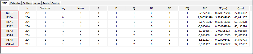
The results presented by the Matrix node
Seasonality tests
The Diagnostics node includes a set of seasonality tests that are useful for checking for the presence of seasonality in the time series. The tests are described in the Seasonality tests sections. The tests check for the presence of seasonality in:
-
The original series (log transformed, if necessary);
-
Linearised series;
-
Full residuals;
-
SA series;
-
Irregular;
-
Residuals (last periods);
-
SA series (last periods);
-
Irregular (last periods);
Seasonal adjustment should be applied only to the seasonal series. However, regression effects can mask the underlying seasonal pattern. Therefore, seasonality should be statistically significant in the linearised series. Finally, seasonally adjusted series should not have neither residual seasonality nor residual calendar effects and should show both the full trend and irregular component.8 The presence of seasonality can also be checked by the combined seasonality test, which originates from the X-11 algorithm and considers the results of several seasonality tests to judge if the series manifests identifiable seasonal fluctuations.
Spectral analysis
Seasonal and calendar effects are approximately periodic, therefore the spectrum is an appropriate tool to reveal their presence9. The periodicity of phenomenon at frequency \(f\) is\(\ \frac{2\pi}{f}\). It means that for a monthly time series the seasonal frequencies are: \(\frac{\pi}{6},\ \frac{2\pi}{6},\ \frac{3\pi}{6},\ \frac{4\pi}{6},\ \frac{5\pi}{6},\ \pi\) (which are equivalent to cycles per year i.e. in the case of a monthly series, the frequency \(\frac{2\pi}{6}\) corresponds to a periodicity of 6 months (2 cycles per year are completed)). For a quarterly series there are two seasonal frequencies: \(\frac{\pi}{2}\) (one cycle per year) and \(\pi\) (two cycles per year). A peak at the zero frequency always corresponds to the trend component of the series. For more details about spectral analysis see here.
JDemetra+ displays the spectral plots obtained for two spectrum estimators: periodogram and autoregressive spectrum10. They are intended to alert to the presence of remaining seasonal and trading day effects. The graphics are available for the residuals, the irregular component and the seasonally adjusted time series. Seasonal frequencies are marked as blue vertical lines, while red lines represent the trading day effect frequencies. The \(X\)-axis shows the frequencies from 0 to \(\pi\).
The interpretation of the spectral graph is rather straightforward. When the values of a spectral graph for low frequencies are large in relation to the other values, than the long-term movements dominate in the series. When the values of a spectral graph for high frequencies are large in relation to its other values, then the series is rather trendless and contains a lot of noise. When the values of a spectral graph are distributed randomly around a constant without any visible peaks, then it is highly probable that the series is a random process. The presence of seasonality in a time series is manifested by the peaks at the seasonal frequencies, while the peaks at the trading day frequencies correspond to the presence of a trading day effect. The explanations for the trading day frequencies are given in here.
At the seasonal and trading day frequencies, a peak in the residuals indicates the need for fitting a better model. In particular, peaks at the seasonal frequencies are caused by inadequate filters chosen for the decomposition. Peaks at the trading day frequencies could occur due to inappropriate regression variables used in the model.
A peak in the spectrum of the seasonally adjusted series or irregulars reveals inadequacy of the seasonal adjustment filters for the time interval used for spectrum estimation. In this case a different model specification or a different length of a data span should be considered.
If at least one significant peak (\(Pvalue > 0.05\)) has been detected in the residuals, JDemetra+ displays a green line that denotes the \(0.05\ \)significance level. Peaks above this limit are considered to be significant at the \(0.05\ \)significance level11.
An autoregressive spectrum graph available in JDemetra+ is based on the relevant tool from the X-13ARIMA-SEATS program. It shows the spectral density (spectrum) function, which reformulates the autocovariances of the stationary time series in terms of amplitudes at frequencies of half a cycle per month or less.
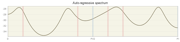
Autoregressive spectrum for residuals from the TRAMO model
The periodogram is one of the earliest tools used for the analysis of time series in the frequency domain. It enables the user to identify the dominant periods (or frequencies) of a time series. In general, the periodogram is a wildly fluctuating estimate of the spectrum with a high variance and is less stable than the autoregressive spectrum12.
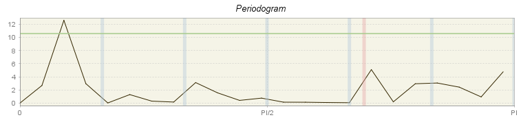
Periodogram for residuals from TRAMO model
For computational reasons none of the periodograms for seasonally adjusted series and for the irregular displays the line that indicates the peaks above the \(0.05\ \)significance level. Therefore, there is no message if the peaks visible on those panels are significant or not.
Standard Copy/Print/Export options are avaiable for these charts.
Sliding spans
Seasonally adjusted time series are expected to be stable, which means that they do not change substantially when removing or adding few data points to the original series. This characteristic is assessed by the sliding spans13 analysis. This tool can be also used to detect significant changes in the original time series, such as seasonal breaks14, large number of outliers and fast moving seasonality15.
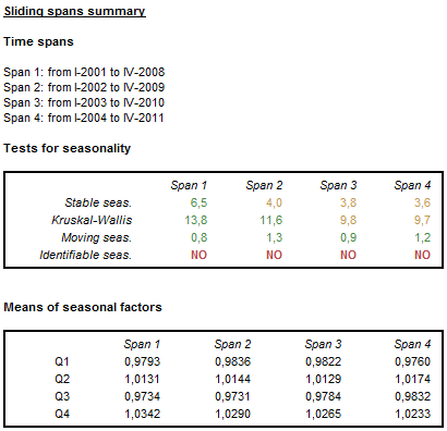
A sliding spans analysis uses the concept of a span, which is defined as a range of data between two dates. The sliding spans are series of two, three or four (depending on the length of the original time series) overlapping spans. The algorithm sets up a maximum of 4 spans, the length of each span is always 8 years16. The spans start in 1 year intervals.
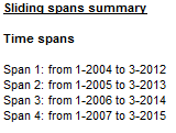
The list of spans used in the analysis
The sliding spans analysis compares the seasonally adjusted values for a given observation, obtained by applying the seasonal adjustment procedure to the consecutive spans. Each period (month or quarter), that is common to more than one span, is examined to see if its seasonal adjustments vary more than a specified amount across the spans.
The summary of the sliding spans includes the results of several seasonality tests for each span. The differences between spans signal the change in the characteristic of seasonal movements in the time series. For the description of the seasonality tests see here.
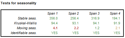
The results of the tests for seasonality performed for a set of spans
The differences in the mean of seasonal factors between different spans observed for a given period signal a potential change in the characteristic of the seasonal fluctuations.
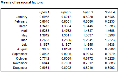
Means of seasonal factors for the consecutive spans
JDemetra+ performs sliding spans analysis not only for seasonally adjusted series, but also for the trading day/working day effect (if present) and the seasonal component. The detailed results are displayed in the sub-nodes: Seasonal, Trading days and SA (changes). The later panel is related to the period-to-period percentage changes in seasonally adjusted series. The threshold value to detect abnormal values is set to 3% of the testing statistics. The respective formulas are given in the Seasonality tests sections. In this section the standard Copy/Print/Export options are available only for graph that presents the sliding spans statistics.
The layout of each of these sub-nodes is the same. The explanations provided here for the seasonal component can be adapted accordingly to the other two sub-nodes. The user should be aware that an unstable estimate of a seasonal factor for a given period can give rise to unstable estimates of the two associated period-to-period changes. Because of that, in the majority of cases, more months are flagged for unreliable period-to-period changes than for unreliable seasonal factors17.
The first panel shows the sliding spans statistics calculated for each period. For the given period the sliding spans statistic is the maximum percentage difference between the estimates of the seasonal component obtained from different spans. The estimation of seasonal component is regarded as unstable if this statistic is greater than 3%.
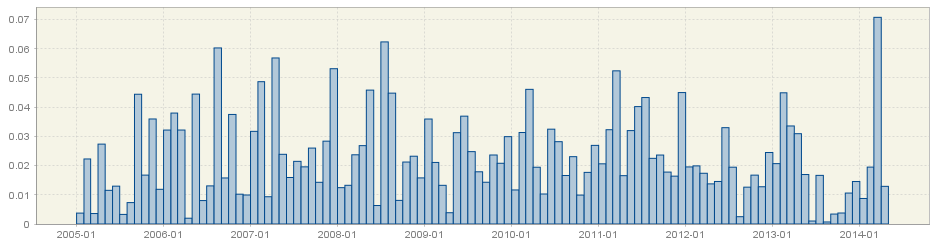
The sliding spans statistics for the seasonal component
The next panel presents the cumulative frequency distribution of the sliding spans statistics (months or quarters) using the frequency polygon. On the horizontal axis the values of the sliding spans statistics are shown, while the vertical axis presents the frequency (in percentages) of each class interval18. For a distribution shown in the figure below the first interval extends from 0 to 0.005. This interval has a frequency 9%, which means that 9% of the sliding spans statistics are in this interval.
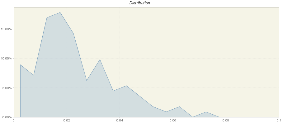
The cumulative frequency distribution of the sliding spans statistics
According to FINDLEY, D., MONSELL, B.C., SHULMAN, H.B., and PUGH, M.G. (1990), the results of seasonal adjustment are stable if the percentage of unstable (abnormal) seasonal factors is less than 15% of the total number of observations. Empirical surveys support the view that seasonal adjustments with more than 25% of the months (or quarters) flagged for unstable seasonal factor estimates are not acceptable17. Therefore, the user should check for the total frequency of the intervals between 0.03 and 1.
The last panel contains detailed information about the percentage of values that exceed the threshold value (0.03) and therefore are considered to be abnormal. In the example presented in the figure below, 28.6% of values have been marked by the sliding spans diagnostic as abnormal.
JDemetra+ also provides information about the number of breakdowns of unstable factors and average maximum percentage differences grouped by month (or quarter) and by year. It gives an idea of whether observations with unreliable seasonal adjustment values cluster in certain calendar periods and whether their sliding spans statistics barely or substantially exceed the threshold value. The figure below presents that three sliding spans statistic calculated for January are above 3% and that the average maximum percentage difference across spans for this period was 2.0.
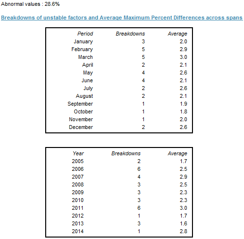
Breakdowns of unstable factors and average maximum percent differences across spans
Sliding spans analysis is a tool that can be used for correcting the model. For example, a large number of unstable estimates revealed by the sliding spans analysis indicates that the model specification may need to be changed. Comparing the seasonality tests results for consecutive spans may also indicate that the seasonal pattern has changed substantially. In such case the user should investigate this issue further and decide wether to reduce the time series span.
Sliding span summary for the series, for which the seasonal fluctuations fade away
Revision histories
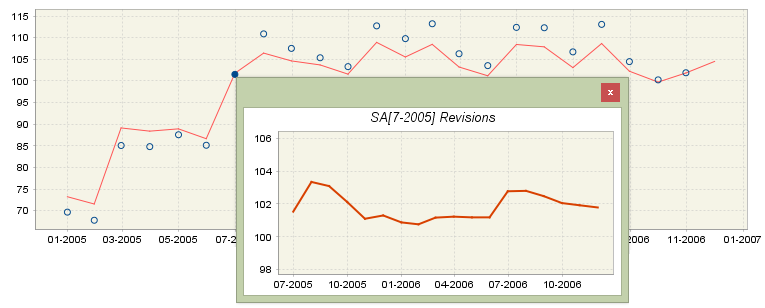
It is well-known that the seasonally adjusted and trend estimates change as new observations are added to the end of the original time series. The changes in the estimated SA and trend values are called revisions and can be analysed with the tool called Revision history. JDemetra+ illustrates differences between the initial estimate (marked by a blue circle) and the latest estimate (red line). A revision is defined as a difference between these two values. As a rule, smaller revisions are better.
The revision history is useful for comparing results from competing models. When the user defines two seasonal adjustment models for one time series and both these models are acceptable, the revision history can be used for choosing a better model in terms of revisions. However, it is not an actual statistical test but a complementary descriptive analysis.
JDemetra+ generates revisions between the initial estimate and the most recent estimate for the seasonally adjusted series, the trend components as well as for month-to-month (or quarter-to-quarter) changes in the seasonally adjusted series and in the trend.
The revision history is performed for the maximum of 84 most recent observations (monthly series) or 16 most recent observations (quarterly series). When a time series is shorter than 109 observations (monthly series) or 37 observations (quarterly series) the number of data points considered by the revision history analysis is reduced accordingly. For series shorter than 62 observations (monthly series) or 22 observations (quarterly series) the revision history is not computed.
Revision history results
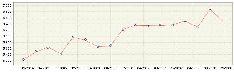
If the user clicks on a blue circle, which represents the initial estimation for period \(t_{n}\), an auxiliary window will appear. This additional figure shows the successive estimations (computed on \(\left\lbrack t_{0},\ \ldots,t_{n} \right\rbrack\), \(\left\lbrack t_{0},\ \ldots,t_{n + 1} \right\rbrack,\ \ldots,\left\lbrack t_{0},\ \ldots,t_{T} \right\rbrack\) of the considered series for the period \(t_{n}\). With this figure the user can evaluate how the seasonally adjusted observations have changed from the initial to the final estimation. The analogous graph is available for the trend analysis.
Revision history results – insight into successive estimations for the given period
By looking at the vertical axis the user could assess the size of the revision. The revisions presented in the figure above are about 2% (103 - 101 = 2). The figure size can be enlarged by dragging the bottom-right corner.
For the seasonally adjusted series and for the trend component the revision history analysis plot is accompanied by information about the relative differences between the initial and the final estimates for the last four years. For the changes in seasonally adjusted series and in the trend the period to period growth rates instead of relative differences are displayed. For an additive decomposition the absolute revisions are used. For a multiplicative decomposition the relative differences are considered. Values, which are larger (in absolute terms) than two times the root mean squared error of the (absolute or relative) revisions, are marked in red and provide information about the instability of the output. Information about the mean relative difference between the initial and the final estimation over a period displayed in the table is also provided. As relative differences can be positive as well as negative, the mean value is not very informative for detecting any possible bias. The magnitude of varying revisions is measured by the root mean square error (RMSE), which has the same units as the mean.
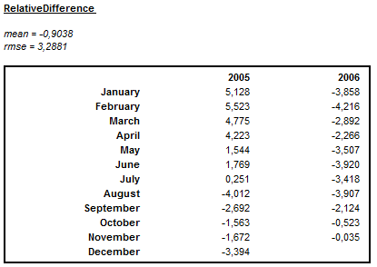
Summary of the size of the revisions for a multiplicative decomposition
The revision history provides no absolute measure of what is an acceptable level of revisions. Therefore the revision history is of limited use on a single series. More information about the revision history is available here.
Model stability
The diagnostics output window provides some purely descriptive features, which can be used to analyse the stability of the parameters of the TRAMO model, including the trading/working day effect, the Easter and the ARIMA part. The model stability analysis estimates the coefficients of the TRAMO model applied for 8 years long spans. The number of estimations depends on the length of the series. For example, when the series is 12 years long, then only five estimations will be calculated. The points displayed in the figure correspond to the successive estimations.
The figures displayed in this section are useful for assessing the stability of the model parameters. The first panel presents estimation results for one (working day effect) or six (trading day effect) regression coefficients. The graph is not displayed when none of these effects is included in the TRAMO model.
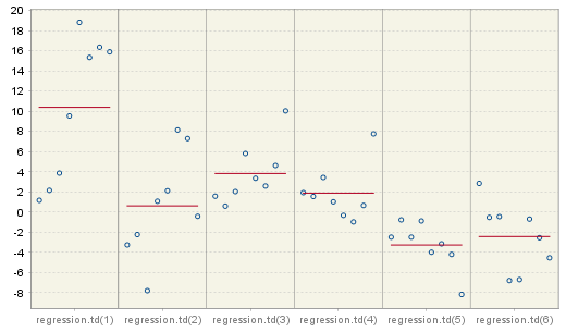
Estimation parameters for the trading day effect
The concentration of the estimation results (denoted by blue circles) around the mean (red, horizontal line) indicates the stability of the results in time. In the case presented in the figure below however, the values of the Easter effect parameters vary from 2.5 to -3.5, indicating the instability of the results and potential insignificance of this effect.
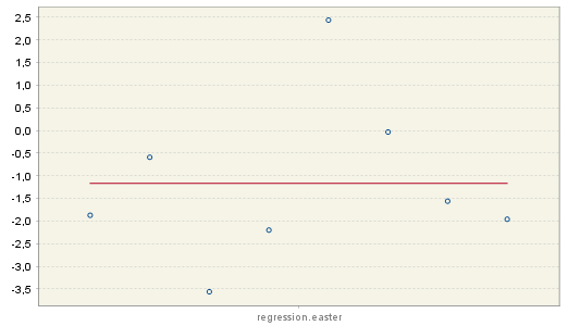
Estimation parameters for the Easter effect
The results from the estimation of an ARIMA (3,1,0)(0,0,1) model over 8 spans, which is shown in the figure below, reveal quite high stability of the estimations.
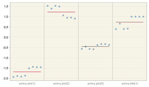
Estimation parameters for the ARIMA model
The user can enlarge the results for a given parameter. It can be done by double clicking on the area of interest. The details are displayed in a resizable pop-up window (double right click to the restore the default view).
Multi-processing
The Multi processing section, which belongs to the Seasonal adjustment node, is designed to store the results of the seasonal adjustment procedure performed with the TRAMO-SEATS or X-13ARIMA-SEATS methods. The Multi processing is designed for a quick and efficient seasonal adjustment of large data sets using different seasonal adjustment methods and different specifications. The functionality is activated from the main menu.
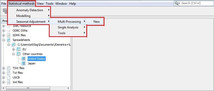
Launching a seasonal adjustment process for a dataset
The default specification used for multi-documents can be set in the Tools → Options item from the main menu, where the user is expected to specify the seasonal adjustment specification in the Statistics panel.
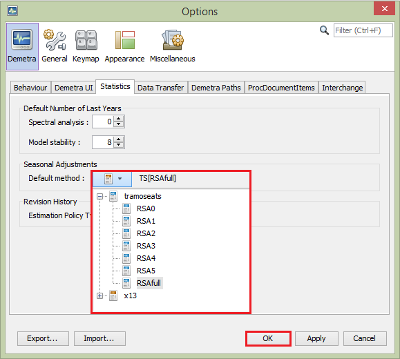
Specifying the default seasonal adjustment method
The consecutive steps necessary to launch the seasonal adjustment process for a dataset are described in this case study. The in-depth analysis of seasonal adjustment results and possible ways to correct the deficiencies of the specification and improve the modelling are given throughout the Case studies sections.
Within one multi-document the user may apply different specifications to the different time series and/or perform the seasonal adjustment for a given time series using different specifications in order to compare the results.
The multi-document window (called the SAProcessing-#number window) consists of three panels. The first one – Processing – presents the list of the series. Once the seasonal adjustment process is launched, concise information about the quality of the results is displayed in the Quality column and major problems are manifested in the Warnings column. When the user clicks on an individual time series in the SAProcessing-#number window, detailed results are displayed in the panel below the list of series. By default, a summary of results is displayed, accompanied by two graphs: the original data, seasonally-adjusted series and trend on the left and the SI ratios on the right. All the options available for this panel, including launching the seasonal adjustment process, are presented here and here.
The Processing panel view
The Summary panel gives general information on the results of the adjustment. The report is organised into sections corresponding to the SA methods and frequencies of the time series (monthly and quarterly), which are available from the menu on the top of the panel. The example below shows that the X-13ARIMA-SEATS method has been applied to the three monthly time series. All of them have been logarithmically transformed. The list of the ARIMA models shows the models’ parameters used in the seasonal adjustment process of the dataset. There were 6 outliers detected, the majority of which were additive outliers. Calendar effects haven’t been detected for any of the time series seasonally adjusted with the X-13ARIMA-SEATS method.
The Summary panel view
The last panel – Matrix view panel – provides information similar to the matrix output of TSW+ (TRAMO-SEATS for the Windows program).
The Matrix panel view
Footnotes
-
MARAVALL, A., CAPORELLO, G., PÉREZ, D., and LÓPEZ, R. (2014). ↩ ↩2
-
The series is deterended with the Hodrick-Prescott filter. ↩ ↩2
-
See Linearization section. ↩ ↩2
-
FINDLEY, D., MONSELL, B.C., BELL, W.R., OTTO, M.C., and CHEN, B.-C. (1990). Basic information about spectral analysis is presented in 7.3. ↩ ↩2
-
The theoretical motivation for the choice of spectral estimator is provided by SOKUP, R., and FINDLEY, D. (1999). ↩ ↩2
-
This indicator appears only if the series is a white noise (residuals) as the periodogram is then distributed as a \(\chi^{2}\). ↩ ↩2
-
For description of the periodogram see Periodogram. The autoregressive spectrum is discussed here. ↩ ↩2
-
See Sliding spans. ↩ ↩2
-
A seasonal break is defined as a sudden and sustained change in the seasonal pattern of a series. The presence of this event is reflected in SI ratio. A seasonal break is an unwanted feature of the time series as the moving averages used by X-1-ARIMA are designed to deal with series, which have a smoothly evolving ‘deterministic’ seasonal component plus an irregular component with a stable variance. ↩ ↩2
-
Fast moving seasonality means that the seasonal pattern displays rapidly evolving fashion from year to year. ↩ ↩2
-
The procedure of withdrawing spans from time series is described in FINDLEY, D., MONSELL, B.C., SHULMAN, H.B., and PUGH, M.G. (1990) as follows: to obtain sliding spans for a given series, an initial span is selected whose length depends on the seasonal adjustment filters being used. A second span is obtained from this one by deleting the earliest year of data and appending the year of data following the last year in the span. A third span is obtained from the second in this manner, and a fourth from the third, data permitting. This is done in such a way that the last span contains the most recent data. ↩ ↩2
-
FINDLEY, D., MONSELL, B.C., SHULMAN, H.B., and PUGH, M.G. (1990). ↩ ↩2 ↩3 ↩4
-
In frequency polygon data presented on the horizontal axis are grouped into class intervals. ↩ ↩2
-
See Estimation of the components with the Wiener-Kolmogorow filter in the SEATS section. ↩
-
PLANAS, C. (1998). ↩
-
See PsiE-weights in the SEATS section. For further details see MARAVALL, A. (2008b). ↩
-
GÓMEZ, V., and MARAVALL, A. (2001). The current adjustment means that model, filters, outliers and regression parameters are re-identified and the respective parameters and factors re-estimated at appropriately set review periods (usually once a year). The seasonal and calendar factors to be used to adjust for seasonal and calendar effects of new unadjusted data in-between the review periods are those estimated in the previous review period and forecasted up to the next review period. In the concurrent adjustment strategy the model, filters, outliers, regression parameters are re-identified and the respective parameters and factors re-estimated every time new or revised data become available. Source: ‘ESS Guidelines on Seasonal Adjustment’ (2015). ↩
-
The variance of the component innovation is the variance resulting from the ARIMA model for this component. ↩
-
KAISER, R., and MARAVALL, A. (2005). ↩
-
MARAVALL, A. (1997). ↩
-
From the TRAMO-SEATS estimator structure it can be shown that the estimator will always underestimate the component. The amount of the underestimation depends on the particular model and as a rule the relative underestimation will be large when the variance of the component is relatively small, MARAVALL, A. (1995). ↩
-
The theoretical variance (Estimator) should be similar to the estimate actually obtained (Estimate). Large differences between the theoretical and empirical values would indicate misspecification of the overall model, MARAVALL, A. (1995). ↩
-
See Autocorrelation and partial autocorrelation functions here. ↩
-
DAGUM, E.B. (1987). ↩