Options for the RegArima specifications

This section discusses the options available for the RegARIMA specifications, which are based on the original X-13ARIMA-SEATS program developed by the U.S. Census Bureau.

The options available for the RegARIMA specifications are divided into five parts. These sections are:

• Estimate;
• Transformation;
• Regression;
• Outliers;
• Arima.

The RegARIMA specifications are to a very large extent organised according to the different individual specifications of the original program and are presented in the order in which they are displayed in the graphical interface of JDemetra+.

The RegARIMA specification sections

To facilitate the comparison between JDemetra+ specifications and specifications used in Win X-13, under each option the name of the corresponding specification and argument from the original software is given, if any. For an exact description of the different parameters, the user should refer to the documentation of the original X-13ARIMA-SEATS program¹. Some additional explanations about the RegARIMA model, its parameters and estimation procedure are given here.

For the pre-defined specifications the parameters are fixed, but in the case of the user-defined specification the user can set them individually. However, as in some cases the choice of a given value results in limitation of the possible alternatives for other parameters, the user is not entirely free to set the values of the parameters. Most arguments have default values; these are given in the documentation and used unless changed by the user.

Estimate

The Estimate section specifies the details of estimation procedure of the RegARIMA model determined in the Regression and Arima sections.

RegARIMA specification – options for the Estimate section

• Model span $\rightarrow\ $type
  series {modelspan}

  Specifies the span (data interval) of the time series to be used for the estimation of the RegARIMA model coefficients. The RegARIMA model is then applied to the whole series. With this argument the data early in the series can be prevented from affecting the forecasts, or, alternatively, data later in the series are excluded from the modelling span, so that they do not influence the regression estimates. The available parameter values are:

  • All – full time series span is considered in the modelling;
  • From – date of the first time series observation is included in the pre-processing model;
  • To – date of the last time series observation is included in the pre-processing model;
  • Between – dates of the first and the last time series observations are included in the pre-processing model;
  • Last – a specific number of observations from the end of the time series is included in the pre-processing model;
  • First – a specific number of observations from the beginning of the time series is included in the pre-processing model;
  • Excluding – a specific number of observations is excluded from the beginning (first) and/or end (last) of the time series in the pre-processing model.

  With the options Last, First, Excluding the span can be computed dynamically on theseries. The default setting is All.

• Tolerance
  estimate {tol}

  Convergence tolerance for the nonlinear estimation. The absolute changes in the log-likelihood function are compared to Tolerance to check for the convergence of the estimation iterations. The default setting is 0.0000001.

Transformation

The Transformation section is used to transform the series prior to estimating the RegARIMA model.

RegARIMA specification – options for the Transformation section

• Function
  transform {function=}

  Transformation of data. ² The user can choose between:

  • None – no transformation of the data;
  • Log – takes logs of the data;
  • Auto – the program tests for the log-level specification. This option is recommended for automatic modelling of many series.

  The default setting is Auto.

• AIC difference
  transform {aicdiff=}

  Defines the difference in AICC needed to accept no transformation over a log transformation when the automatic transformation selection option is invoked. The option is disabled when Function is not set to Auto. The default AIC difference value is -2.

• Adjust
  transform {adjust=}

  Options for proportional adjustment for the leap year effect. The option is available when Function is set to Log. Adjust can be set to:

  • LeapYear – performs a leap year adjustment of monthly or quarterly data;
  • LengthofPeriod – performs a length-of-month adjustment on monthly data or length-of-quarter adjustment on quarterly data;
  • None – does not include a correction for the length of the period.

  The default setting is None.

Regression

The Regression section allows for estimating deterministic effects in the series with the pre-defined regression variables. These variables include user-defined variables, several types of pre-specified outliers, intervention variables and calendar effects. The pre-defined and user-defined regression variables are selected with the Variables argument.

RegARIMA specification – options for the Regression section

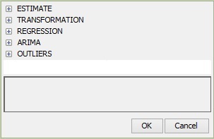
• Calendar $\rightarrow\ $ tradingDays $\rightarrow\ $ option
  regression {variables = td1nolpyear, td, tdnoleapyear, td1coef}

  Specifies the type of calendar being assigned to the series. The following types of calendar estimation are available:

  • None – excludes calendar variables from the regression model.
  • Default – means that a default JDemetra+ calendar, which does not include any country-specific holidays, will be used.
  • Stock – estimates day-of-week effects for inventories and other stock reported for the $w^{\text{th}}$ day of the month (to denote the last day of the month enter 31).
  • Holidays – corresponds to the pre-defined trading day variables, modified to take into account country specific holidays. It means that after choosing this option the user should specify the type of the trading day effect (Calendar $\rightarrow\ $ tradingDays $\rightarrow\ $ TradingDays) and a previously defined calendar that includes the country specific holidays (Calendar $\rightarrow\ $ tradingDays $\rightarrow\ $ holidays).
  • UserDefined – used when the user wants to specify his own trading day variables. With this option calendar effects are captured only by regression variables chosen by the user from the previously created list of user-defined variables.

  The default setting is Default.

  

  The option menu

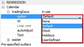
• Calendar $\rightarrow\ $ tradingDays $\rightarrow\ $ holidays
  regression {variables=holiday}

  A list of user-defined calendars to be used to create calendar regression variables. Option is available when Calendar $\rightarrow\ $ tradingDays $\rightarrow\ $ option is set to Holidays. The user is expected to click the field to expand a list a previously defined calendars and choose an appropriate item. The default setting is Default, which implies that the default calendar is used and no country-specific holidays are considered.

  

  The list of calendars displayed under Holidays option corresponds to the calendars defined in the Workspace window

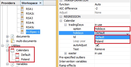
• Calendar $\rightarrow\ $ tradingDays $\rightarrow\ $ userVariables
  regression {variables=}

  A list of predefined regression variables to be included in the model. Option is available when Calendar $\rightarrow\ $ tradingDays $\rightarrow\ $ option is set to UserDefined. When the user chooses the UserDefined type for the trading day effect estimation, one must specify the corresponding variables. It should be noted that such variables must have been previously defined, otherwise the list in the field Calendar $\rightarrow\ $ tradingDays $\rightarrow\ $ userVariables is empty. The default setting is Unsused.

  

  Assigning the user-defined variables to the RegArima model

• Calendar $\rightarrow \ $ tradingDays $\rightarrow \ $ td
  regression {variables=td}

  Assigns a type of model-estimated regression effect to pre-specified regression variables. Option is available when Calendar $\rightarrow\ $ tradingDays $\rightarrow\ $ option is set to Default or Holidays. Acceptable values:

  • None – means that no calendar variables will be included in the regression.
  • TradingDays – includes six day-of-the-week regression variables.
  • WorkingDays – includes the working/non-working day contrast variable.

  The default setting is TradingDays.

  

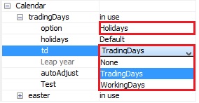
  The trading days menu

• Calendar $\rightarrow\ $ tradingDays $\rightarrow\ $ lp
  regression {variables=lp}

  Includes the leap-year effect in the model. Acceptable values:

  • None – the leap-year effect is not included in the model;
  • LeapYear – includes a contrast variable for the leap-year;
  • LengthofPeriod – includes length-of-month (or length-of-quarter) as a regression variable to model the leap year effect.

  The default setting is LeapYear.

• Calendar $\rightarrow\ $ tradingDays $\rightarrow\ $ autoAdjust

  Option for an automatic correction for the leap year effect. It is available when in the Transformation section function is Auto. By default it is enabled.

• Calendar $\rightarrow\ $ tradingDays $\rightarrow\ $test
  regression; aictest

  Pre-tests the significance of the trading day regression variables using the AICC statistics. The user can choose between the following options:

  • Add – the trading day variables are not included in the initial regression model but they can be added to the RegARIMA model after the test.
  • None – the test is not performed; the specified calendar variables are used in the model without pre-testing.
  • Remove – the trading day variables belong to the initial regression model but they can be removed from the RegARIMA model after the test.

  These options have no direct impact on the calendar tests themselves, but indirectly, through the definition of the regression model, on any previous test. For instance, on rare occasions the log/level test could be affected by add/remove on the trading day effect. The default setting is Remove.

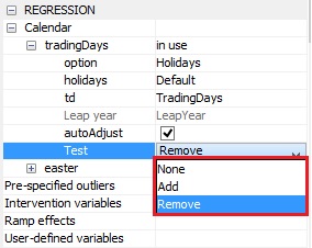
The test menu

• Calendar $\rightarrow\ $ easter $\rightarrow\ $ IsEnabled
  regression; variables and/or aictest

  The option enables the user to consider the Easter effect in the RegARIMA model. When the user ticks this option it means that the correction for the Easter effect is considered. The inclusion of the Easter effect in the model depends on the choice made in the Pretest section. Otherwise a correction for the Easter effect is not performed.

• Calendar $\rightarrow \ $ easter $\mathbf{\rightarrow}$ Use Julian Easter

  When marked, it enables Easter to be included, the date of which is derived from the Julian calendar and is converted to Gregorian calendar date. By default, the checkbox is unmarked.

• Calendar $\rightarrow\ $ easter $\rightarrow\ $ Pre-test
  regression; aictest

  Pre-tests the significance of the Easter regression variable using the AICC statistics. The user can choose between the following options:

  • Add – the Easter effect is not included in the initial regression model but it can be added to the RegARIMA model after the test.
  • None – the Easter effect is not pre-tested.
  • Remove – the Easter effect belongs to the initial regression model and it can be removed from the RegARIMA model after the test.

  These options have no direct impact on the calendar tests themselves, but indirectly, through the definition of the regression model, on any previous test. For instance, on rare occasions the log/level test could be affected by add/remove on the Easter effect. The default setting is Add.

• Calendar $\rightarrow \ $ easter $\rightarrow \ $ Easter duration
  regression {variables = easter[w]}

  Duration (length in days) of the Easter effect. The length of the Easter effect can range from 1 to 20 days.³ The Easter duration option is displayed when Calendar $\rightarrow\ $ easter $\rightarrow\ $ Pre-test is set to either None or Remove. The default value is 8.

• Pre-specified outliers
  regression {variables = (ao tc ls so)}

  User-defined outliers are used when prior knowledge suggests that certain effects exist at known time points.⁴ Four pre-defined outlier types, which are simple forms of intervention variables, are implemented:

  • Additive Outlier (AO);
  • Level shift (LS);
  • Temporary change (TC)⁵;
  • Seasonal outliers (SO).

  Descriptions and formulas are available in Linearisation with the TRAMO and RegARIMA models. By default, no pre-specified outlier is included in the specification.

• Intervention variables
  regression {user=}

  The intervention variables are defined as in TRAMO. Following the definition, these effects are special events known a priori (strikes, devaluations, political events, and so on). Intervention variables are modelled as any possible sequence of ones and zeros, on which some operators may be applied. Intervention variables are built as combinations of the following basic structures:⁶

  • Dummy variables⁷;
  • Any possible sequence of ones and zeros;
  • $\frac{1}{(1 - \delta B)}$, $(0 < \delta \leq 1)$;
  • $\frac{1}{(1 - \delta_{s}B^{s})}$, $(0 < \delta_{s} \leq 1)$;
  • $\frac{1}{(1 - B)(1 - B^{s})} $; where $B$ is a backshift operator (i.e. $B^{k}X_{t} = X_{t - k}$) and $s$ is frequency of the time series ($s = 12\ $for a monthly time series, $s = 4\ $for a quarterly time series).

  These operations enable not only AO, LS, TC, SO and RP outliers to be generated, but also sophisticated intervention variables that are well-adjusted to the particular case. No intervention variables are included in the pre-defined specifications. They can only be added to the user-defined specifications.Intervention variables are not implemented in X-13ARIMA-SEATS, however they can be created by the user and introduced to the model as user-defined variables.

• Ramp effects
  regression {variables = (rp)}

  A ramp effect means a linear increase or decrease in the level of the series over a specified time interval $t_{0}$ to $\ t_{1}$. All dates of the ramps must occur within the time series span. Ramps can overlap other ramps, additive outliers and level shifts. The graph and formula are available in Linearisation with the TRAMO and RegARIMA models. No ramps are included in the pre-defined specifications. They can only be added to the user-defined specifications.

  

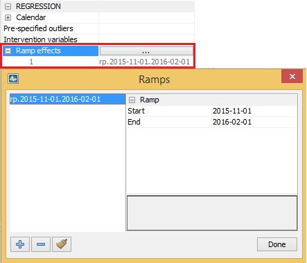
  Defining the Ramp effects

• User-defined variables
  regression {user=}

  The user-defined variable is an external regressor included by the user in the RegARIMA model. To add a user-defined variable to the model, one must specify the corresponding variable in the Variables window. First, click the Unnamed item and then click the Name field to expand a list of available variables and choose a variable from the list. It should be noted that such variables must have been previously defined (see instructions provided here), otherwise the list is empty.

  

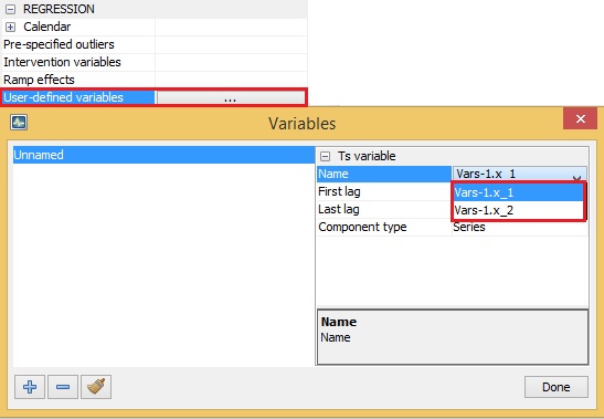
  Defining the user-defined variable

  The user-defined regression variable associated to a specific component should not contain effects that have to be associated with another component. Therefore, the following rules should be obeyed:

  • The variable assigned to the trend or to the seasonally adjusted series should not contain a seasonal pattern;
  • The variable assigned to the seasonal should contain neither a trend nor a level (i.e. should have a zero mean);
  • The variable assigned to the irregular should contain neither a seasonal pattern nor a trend (i.e. should have a zero mean);

  The user-defined variables should cover the period of the dependent series and the appropriate number of forecasts. For the other periods the variables are implicitly set to 0. If the forecasts are not provided, it will not alter the results of the seasonal adjustment but the forecasts of the final components will be unusable. The effect of the user-defined variable can be assigned to the:

  • Series;
  • Trend;
  • Irregular component;
  • Seasonal component;
  • Seasonally adjusted series;
  • Series;
  • Undefined (a default setting), which implies that the effect is an additional component ⁸. With this option the regression variable is used to improve the modelling, but it is not removed from the series for the decomposition⁹.

  The calendar component is not available in this section. Therefore, a user-defined variable assigned to the calendar effect should be added in the calendar part of the specification. For the user-defined variable the structure of the lags can be specified using the options first lag and last lag¹⁰. When the regression variable $x_{t}$ is introduced with first lag = and last lag =, JDemetra+ includes in the TRAMO model a set of variables $x_{t - l_{a}}$,…,$\ x_{t - l_{ b}}$ and estimates the respective regression coefficients called the impulse response weights. To include only the first lag ($x_{t - 1})\ $ of the user-defined variable ($x_{t})\ $in the RegARIMA model the user should put first lag = last lag = 1. If for a monthly series one puts first lag = 0 and last lag = 11, it means that in addition to instantaneous effect of the user-defined variable, also the effects of 11 lagged explanatory variables are included in the model. In this case the set of estimated coefficients, called a transfer function, describe how the changes in $x_{t}$ that took place over a year are transferred to the dependent variable. However, the lagged variables are often collinear so that caution is needed in attributing much meaning to each coefficient¹¹. No user-defined variables are included in the pre-defined specifications. They can only be added to the user-defined specifications.

• Fixed regression coefficients
  estimate; fix

  For the pre-specified regression variables this option specifies the parameter estimates that will be held fixed at the values provided by the user. To fix a coefficient the user should undertake the following actions:

  • Choose the transformation (log or none).
  • Define some regression variables in the Regression section.
  • Push on the fixed regression coefficients editor button in the User-defined variables row.
  • Select the regression variable from the list for which the coefficient will be fixed.
  • Save the new settings with the Done button.

  

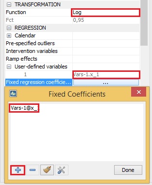
  Fixing the coefficient of the user-defined variable

Outliers

The Outliers section enables the user to perform an automatic detection of additive outliers, temporary change outliers, level shifts, seasonal outliers, or any combination of the four, using the specified model.

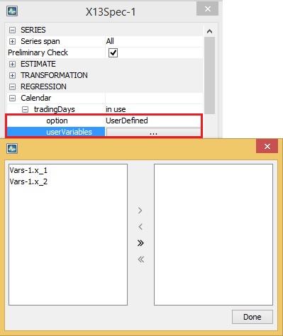
RegARIMA specification – options for the Outliers section

• Is enabled
  outlier; –

  Enables/disables the automatic detection of outliers in the span determined by the Detection span option. By default, the checkbox is marked, which implies that the automatic identification of outliers is enabled.

• Detection span $\rightarrow\ $ type, outlier; span

  A span of the time series to be searched for outliers. The available parameter’s values are:

  • All – full time series span is considered in the modelling;
  • From – date of the first time series observation included in the pre-processing model;
  • To – date of the last time series observation included in the pre-processing model;
  • Between – date of the first and the last time series observations included in the pre-processing model;
  • Last – number of observations from the end of the time series included in the pre-processing model;
  • First – number of observations from the beginning of the time series included in the pre-processing model;
  • Excluding – number of observations excluded from the beginning (specified in the First field) and/or end (specified in the Last field) of the time series in the pre-processing model.

  With the options Last, First, Excluding the span can be computed dynamically on the series. The default setting is All.

• Use default critical value
  outlier; critical

  The critical value is automatically determined by the number of observations in the interval specified by the Detection span option. When Use default critical value is disabled, the procedure uses the critical value inputted in the Critical value item (see below). Otherwise, the default value is used (the first case corresponds to Critical value = "xxx"; the second corresponds to a specification without the critical argument). It should be noted that it is not possible to define a separate critical value for each outlier type. By default, the checkbox is marked, which implies that the automatic determination of the critical value is enabled.

• Critical value
  outlier; critical

  The critical value used in the outliers’ detection procedure. The option is active once Use default critical value is disabled. By default, it is set to 4.0.

• Additive
  outlier; ao

  Automatic identification of additive outliers. By default, this option is enabled.

• Level shift
  outlier; ls

  Automatic identification of level shifts. By default, this option is enabled.

• Transitory change
  outlier; tc

  Automatic identification of transitory changes. By default, this option is enabled.

• Seasonal outlier
  outlier;

  Automatic identification of seasonal outliers. By default, this option is disabled.

• TC rate, outlier; tcrate

  The rate of decay for the transitory change outlier. It must be a number greater than zero and less than one. The default value is 0.7.

• Method
  outlier; method

  Determines how the program successively adds detected outliers to the model. At present only one method, namely AddOne is supported. Using this approach JDemetra+ calculates t-statistics for each type of outlier specified (AO, TC and/or LS) at all time points, for which outlier detection is being performed. If the maximum absolute outlier t-statistic exceeds the critical value, then an outlier has been detected and the appropriate regression variable is added to the model.
  The program then estimates the new model (the old model with the detected outlier added) and searches for an additional outlier. This process is repeated until no additional outliers are found. At this point, a backward deletion process is used to delete outliers, for which the absolute t-statistics no longer exceed the critical value, from the model. This is done one at a time beginning with the least significant outlier, until all outliers remaining in the model are significant. During backward deletion the usual (non-robust) residual variance estimate is used, which can yield somewhat different outlier t-statistics from those obtained during outlier detection.

Arima

An identification of the ARIMA part of the RegARIMA model can be done either in an automatic way or by the user who specifies the appropriate parameters. This choice is controlled by the Automatic option and results in a list of parameters dedicated for chosen ARIMA identification procedure. When the Automatic option is marked, the order of the ARIMA model results from the automatic identification procedure selects the final structure of the ARIMA model. The maximum orders of the regular polynomials are 3, and the maximum orders of seasonal polynomials are 1. The parameters available for automatic model identification are presented below.

RegARIMA specification - options for the automatic identification of the ARIMA model

• Automatic
  automdl; –

  When marked it enables automatic modelling of the ARIMA model to be performed.

• Accept Default
  automdl; acceptdefault

  Controls whether the default model (ARIMA(0,1,1)(0,1,1)) is chosen if the Ljung-Box Q-statistics for these model residuals is acceptable. If the default model is found to be acceptable, no further attempt will be made to identify a model or differencing order. By default, the Accept Default checkbox is unmarked.

• Cancelation limit
  automdl; –

  Cancellation limit for the AR and the MA roots to be assumed equal. This option is mainly used in the automatic identification of the differencing order. The default parameter value is 0.1.

• Initial UR (Diff.)
  automdl; –

  The threshold value for the initial unit root¹² test in the automatic identification of differencing order procedure. When one of the roots in the estimation of the (2,0,0)(1,0,0) plus mean model, which is performed in the first step of the automatic model identification procedure, is larger than First unit root limit, in modulus, it is set equal to unity. The default parameter value is 1.0416666666666667.

• Final UR (Diff.)
  automdl; –

  The threshold value for the final unit root test in the automatic identification of differencing order procedure. When one of the roots in the estimation of the (1,0,1)(1,0,1) plus mean model, which is performed in the second step of the automatic model identification procedure, is larger than Final unit root limit, in modulus, it is checked if there is a common factor in the corresponding AR and MA polynomials of the ARMA model that can be cancelled (see Cancelation limit)). If there is no cancellation, AR root it is set equal to unity (i.e. the differencing order increases). The value of Final unit root limit should be smaller than one. The default parameter value is 0.88.

• Mixed
  automdl; mixed

  Controls whether ARIMA models with non-seasonal AR and MA terms or seasonal AR and MA terms will be considered in the automatic model identification procedure. When this option is disabled, a model with AR and MA terms in both the seasonal and non-seasonal parts of the model can be acceptable, provided there are not AR and MA terms in either the seasonal or non-seasonal.

• Balanced
  automdl; balanced

  Controls whether the automatic model procedure will have a preference for balanced models (i.e. models for which the order of the combined AR and differencing operator is equal to the order of the combined MA operator¹³). By default, the Balanced checkbox is unmarked. When it is marked, the same preference as for the TRAMO program is used.

• ArmaLimit
  automdl; armalimit

  The threshold value for t-statistics of ARMA coefficients used for the final test of a model parsimony. If the highest order of the ARMA coefficient has a t-value less than this value in magnitude, JDemetra+ will reduce the order of the model. The value given for ArmaLimit is also used for the final check for the significance of the constant term; if the constant term has a t-value less than ArmaLimit in magnitude, the program will remove the constant term from the set of regressors. The ArmaLimit value should be greater than zero. The default parameter value is 1.

• Reduce CV
  automdl; reducecv

  The percentage by which the outlier critical value will be reduced when the preferred model is found to have the Ljung-Box Q-statistic with an unacceptable confidence coefficient. The parameter should be between 0 and 1, and will only be active when automatic outlier identification is selected. The reduced critical value will be set to (1-ReduceCV)×CV, where CV is the original critical value. The default parameter value is 0.14268.

• LjungBox limit
  automdl; ljungboxlimit

  Acceptance criterion for the confidence intervals of the Ljung-Box Q-statistic. If the Ljung-Box Q-statistic for the residuals of a final model (checked at lag 24 if the series is monthly, 16 if the series is quarterly) is greater than LjungBox limit, the model is rejected, the outlier critical value is reduced, and model and outlier identification (if specified) is redone with a reduced value (see Reduce CV argument). The default parameter value is 0.95.

• Unit root limit
  automdl; urfinal

  The threshold value for the final unit root test. If the magnitude of an AR root for the final model is less than this number, a unit root is assumed, the order of the AR polynomial is reduced by one, and the appropriate order of the differencing (non-seasonal, seasonal) is increased. The parameter value should be greater than one. The default parameter value is 1.05.

When the Automatic checkbox in the Arima section is unmarked, JDemetra+ allows the user to specify the structure of the ARIMA part of the RegARIMA model. Initial values for the individual AR and MA parameters can be specified for the iterative estimation. Also, individual parameters can be held fixed at these initial values while the rest of the parameters are estimated. The options available here correspond to the original X-13ARIMA-SEATS arima spec with some limitations. JDemetra+ does not allow for operators with missing lags. Also the maximum lag is reduced in comparison with Win X-13.

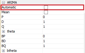
A checkbox for switching bewteen manual and automiatic choice of teh Arima model

JDemetra+ allows the user to fix individual parameters of the ARIMA model at initial values while the rest of the parameters are estimated. However, users should not specify initial values for the MA (moving average) parameters that yield the MA polynomial with the roots inside the unit circle. It is also allowed, e.g. for the iterative estimation, to specify the initial values for the individual AR (autoregressive) and MA parameters.

RegARIMA specification - options for the manual identification of the ARIMA model

• Automatic
  automdl; –

  When unmarked it enables the user to enter the parameters of the ARIMA model.

• Mean
  regression; variables

  When marked t is considered that the mean is part of the ARIMA model (it highly depends on the chosen model).

• P
  arima; model

  The order of the non-seasonal autoregressive polynomial. The maximum order of the non-seasonal autoregressive polynomial is 6. The default value is 0.

• phi
  arima; –

  Coefficients of the non-seasonal autoregressive polynomial (AR). If it is used, a label that indicates the way in which it was estimated should be assigned to each non-seasonal AR parameter in the model. The choice can be made from:

  • Undefined – estimates a parameter without the use of any user defined input (the default value).
  • Initial – estimates a parameter using as initial condition the value defined by the user.
  • Fixed – holds a parameter fixed during estimation at the value defined by the user.

• D
  arima; model

  Non-seasonal differencing order. The maximum number of non-seasonal differences is 2. The default value is 1.

• Q
  arima; model

  The order of the non-seasonal moving average polynomial. The maximum order of the non-seasonal moving average polynomial is 6. The default value is 1.

• theta
  arima; –

  Coefficients of the parameters of the non-seasonal, moving average polynomial (MA). If it is used, a label that indicates the way in which it was estimated should be assigned to each non-seasonal MA parameter in the model. The choice can be made from:

  • Undefined – estimates a parameter without the use of any user defined input (the default value).
  • Initial – estimates a parameter using as initial condition the value defined by the user.
  • Fixed – holds a parameter fixed during estimation at the value defined by the user.

• BP
  arima; model

  The order of the seasonal autoregressive polynomial. The default value is 0.

• Bphi
  arima; –

  Coefficients of the seasonal autoregressive polynomial (AR). If it is used, a label that indicates the way in which it was estimated should be assigned to each seasonal AR parameter in the model. The choice can be made from:

  • Undefined – estimates a parameter without the use of any user defined input (the default value).
  • Initial – estimates a parameter using as initial condition the value defined by the user.
  • Fixed – holds a parameter fixed during estimation at the value defined by the user.

• BD
  arima; model

  Seasonal differencing order. The maximum number of seasonal differences is 1. The maximum order of the seasonal autoregressive polynomial is 4. The default value is 1.

• BQ
  arima; model

  The order of the seasonal moving average polynomial. The maximum order of the seasonal moving average polynomial is 1. The default value is 1.

• btheta
  arima; –

  Coefficients of the parameters of the seasonal moving average polynomial (MA). If it is used, a label that indicates the way in which it was estimated should be assigned to each seasonal MA parameter in the model. The choice can be made from:

  • Undefined – estimates a parameter without the use of any user defined input (the default value).
  • Initial – estimates a parameter using as initial condition the value defined by the user.
  • Fixed – holds a parameter fixed during estimation at the value defined by the user.