Model summary

The Model node includes basic information about the outcome of the model identification procedure and checking the goodness of fit. The summary information about the final model is available directly from the main Model node. The content of this panel depends on the settings applied to the modelling procedure.

The Model node in the navigation tree

The first part contains fundamental information about the model.

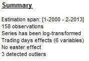
The Summary section of the Model node

Estimation span informs about the first and the last observation used for modelling. The notation of the estimation span varies according to the frequencies (for example, the span [2-1993 : 10-2006] represents a monthly time series and the span [II-1994 : I-2011] represents a quarterly time series). The message Series has been log-transformed is only displayed if a logarithmic transformation has been applied.

In the case of the pre-defined specifications: TR0, TR1, TR3, RG0, RG1 and RG3 no trading day effect is estimated. For TR2, RG2c, TR4 and RG4c pre-defined specifications, working day effects and the leap year effect are pre-tested and estimated if present. If the working day effect is significant, the pre-processing part includes the message Working days effect (1 regressor). The message Working days effect (2 regressors) means that the leap year effect has also been estimated. For TR5 and RG5c the trading day effect and the leap year effect are pre-tested. If the trading day effect has been detected, either of the messages Trading days effect (6 regressors) or Trading days effect (7 regressors) are displayed, depending whether the leap year effect has been detected or not. If the Easter effect is statistically significant, Easter effect detected is displayed.

In this section the total number of detected outliers is displayed. The additional information on detected outliers, i.e. type, location and coefficients’ values, can be found in the Arima model subsection of the Model node.

The Final model section informs about the outcome of the estimation process. Number of effective observations is the number of observations used to estimate the model, i.e. the number of observations of the transformed series (regularly and/or seasonally differenced) reduced by the Number of estimated parameters, which is the sum of regular and seasonal parameters for both autoregressive and moving average processes, mean effect, trading/working day effect, outliers, regressors and one.

Likelihood is a maximized value of a Likelihood¹ function after the iterations processed in Exact Maximum Likelihood Estimation, which is a method used to estimate the model. This value is used by the model selection criteria: AIC, AICC, BIC (corrected by length) and Hannan-Quinn². Standard error of the regression (ML estimate) is the standard error of the regression from Maximum Likelihood Estimation³.

The scores at the solution section presents the gradient of the loglikelihood. The different items of the scores are related to the different parameters of the ARIMA model. The output indicates to which extent the optimization procedure reached the maximum. At the maximum of the likelihood, it should be 0. However, it is never exactly the case, due to numerical approximations. Usually, the scores can be improved by using a higher precision (smaller tolerance). This precision is controlled by the Tolerance parameter in the Estimate section of the Specifications window (see how to use this parameter for Tramo and for Arima).

An example of the output is presented in the chart below.

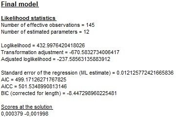
The content of the Final model section

Next, the estimated values of model parameters (Coefficients), t-statistics (T-Stat) and corresponding p-values (P[|T|>t]) are displayed. JDemetra+ uses the following notation:

• Phi(p) – the \(p^{\text{th}}\) term in the non-seasonal autoregressive polynomial;

• Theta(q) – the $q^{\text{th}}$ term in the non-seasonal moving average polynomial;

• BPhi(P) – the $P^{\text{th}}$ term in the seasonal autoregressive polynomial;

• BTheta(Q) – the $Q^{\text{th}}$ term in the seasonal moving average polynomial.

In the example below, the ARIMA model (0,1,1)(0,1,1) was chosen, which means that one regular and one seasonal moving average parameter were identified and estimated. The p-values indicate that BTheta(1) parameter is significant in contrast to the Theta(1), which is not significant ⁴.

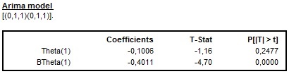
The estimation’s results of the ARIMA model

For the fixed ARIMA parameters, JDemetra+ shows only the values of the parameters. Figure below presents the output from the manually chosen ARIMA model (2,0,0)(0,1,1) with a fixed parameter BTheta(1). For the fixed parameter the T-Stat and (P|T|>t) are not displayed as no estimation is done for this parameter.

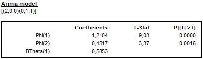
The results of the estimation of the ARIMA model with a fixed coefficient

If the ARIMA model contains a constant term (detected automatically or introduced by the user), the estimated value and related statistics are reported.

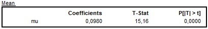
The results of the estimation of a mean effect

JDemetra+ presents estimated values of the coefficients of one or six regressors depending on the type of a calendar effect specification. For a working days effect one regressor is estimated.

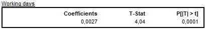
The results of the estimation of a working day effect

When a trading days effect is estimated the Joint F-test value is reported under the table that presents estimated values. When the result of Joint F-test indicates that the trading day variables are jointly not significant the test result is displayed in red.

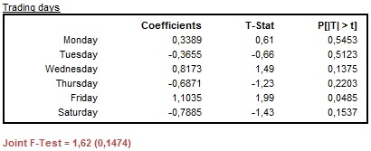
The results of the estimation of a trading day effect: the case of jointly not significant variables

In the example below the RSA5c specification has been used and a trading day effect has been detected. In spite of the fact that some trading day regressors are not significant at the 5% significance level, the outcome of the joint F-test indicates that the trading day regressors are jointly significant (the F-test statistic is lower than 5%).

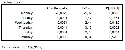
The results of the estimation of a trading day effect: the case of jointly significant variables

If a leap year regressor has been used in the model specification, the value of the estimated leap year coefficient is also reported with the corresponding t-statistics and p-value. As the p-value presented on the picture below is greater than 0.05, it indicates that the leap year effect is not significant.

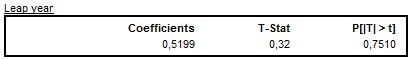
The results of the estimation of a leap year effect

When the option UserDefined is used, JDemetra+ displays the User-defined calendar variables section with variables and corresponding estimation results (the values of the parameters, corresponding t-statistics and p-values). The outcome of the joint F-test is displayed when more than one user-defined calendar variable is used.

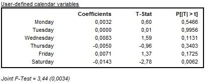
The results of the estimation of user-defined calendar variables

When the Easter effect is estimated, the following table is displayed in the output. In the case presented below Easter has a negative, significant effect on the time series.

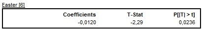
The results of the estimation of the Easter effect

JDemetra+ also presents the results of an outlier detection procedure. The table includes the type of outlier, its date, the value of the coefficient and corresponding t-statistics and p-values.

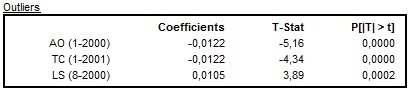
The results of the outlier identification procedure

In all pre-defined specifications, except for TR0 and RG0, only additive outliers, temporary changes and level shifts are considered in the automatic outlier identification procedure. When seasonal outliers are also enabled, they appear in the same table as other outliers.

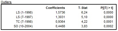
The results of the outlier identification procedure that enables seasonal outliers

Results for pre-specified outliers are displayed in a separate table.

The results of the estimation of the pre-specified outliers

Regression variables, like ramps and intervention variables, are not identified automatically. They need to be defined by the user. The results of an estimation of ramps that are pre-defined types of regression variables are displayed in a separate table. All information concerning ramps, including spans, estimated coefficients and related statistics, is shown in a separate table.

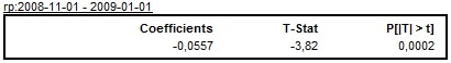
The results of the estimation of the ramp effect

All other intervention variables with corresponding statistics are shown under the Intervention variable(s) table.

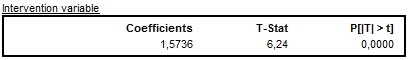
The results of the estimation of the intervention variable

User-defined variables are marked as Vars-1.x_1, Vars-1.x_2, …, Vars-1.x_n and displayed in the separate tables.

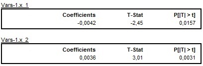
The results of the estimation of the user-defined variables

JDemetra+ also reports a list of missing observations, if any. JDemetra+ applies the AO approach to the estimation of the missing observations⁵.

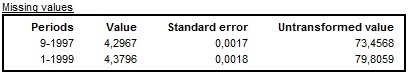
The results of the estimation of the missing observations

Detailed results are divided into several sections and are investigated in the following sections:

• Forecasts
• Regressors
• ARIMA
• Pre-adjustment series
• Residuals
• Likelihood