Forecasts

One of the important steps in of the a validation of the model is an analysis of the out-of-sample forecasts¹. Using the identified TRAMO model JDemetra+ produces the point forecasts, the forecast standard errors, and a prediction interval. The prediction interval on the transformed scale is denoted as$\ point\ forecast \pm K \times forecast\ standard\ error$, where $K$ is the standard error multiplier taken from a table of the normal distribution, corresponding to the specified coverage probability. JDemetra+ displays 95% prediction interval, which corresponds to $K = 1.96.$ The forecasting procedure assumes that no outliers appear in the forecasting period.

The graph presenting time series together with the values forecasted for the next year and corresponding prediction interval can be found directly in the Forecast node.

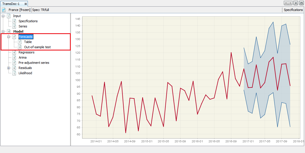
The Forecast panel with visual presentation of the estimated forecasts

The local menu offers the copy and export options, including sending the graph to the printer and save the graph as clipboard or a file in the PNG format. The Show precision gradient option highlights the precision of the estimation using different shades of orange. As a rule, the precision decreases in time, which is depicted by gradually more intense orange. The Copy all series option enables the user to export time series together with the forecasts and the prediction intervals to the another application.

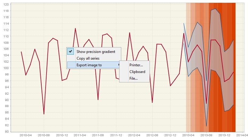
The Forecast panel with visual presentation of the precision of the estimated forecasts

The Forecast node is divided into two subsections: Table and Out-of-sample test. The Table section presents the forecasts as a table.

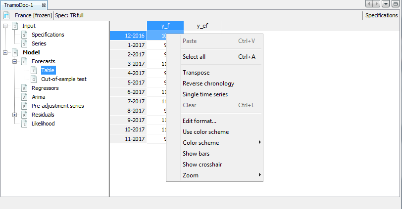
A local menu for the content of the Table panel

A standard local menu, which is available for this table, includes:

• Select all – copies series and allows it to be pasted to the another application e.g. into Excel.

• Transpose – changes the orientation of the table from horizontal to vertical.

• Reverse chronology – displays the series from last to first observation.

• Single time series – when it is marked observations are divided by calendar’s periods. Otherwise, data are presented as a standard time series.

• Edit format – allows changing the format used for displaying dates and values.

• Use color scheme – allows series values to be displayed in colour.

• Color scheme – allows for a choice of colour scheme from a pre-specified list.

• Show bars – presents values in a table as horizontal bars.

• Show crosshair – highlights an active cell.

• Zoom – an option for modifying the chart size.

Paste and Clear are disabled as they are not relevant for this view.

When a time series is marked, a local menu offers the following options:

• Open – opens selected time series in the new window that contain Chart and Grid panels.

• Open with – opens the time series in a separate window according to the user choice (Chart & grid or Simple chart). The All ts views option is not currently available.

• Save – saves the marked series in a spreadsheet file or in a text file.

• Rename – enables the user to change the time series name.

• Copy – copies series and allows it to be pasted to another application e.g. into Excel.

• Paste – pastes the time series previously marked.

• Select all – selects all time series presented in the graph.

• Transpose – changes the orientation of the table from horizontal to vertical.

• Reverse chronology – displays the series from the last to the first observation.

• Single time series – removes from the table all time series apart from the selected one.

• Clear – removes all time series from the chart.

• Edit format – enables the user to change a data format.

• Use color scheme – allows the series to be displayed in colour.

• Color scheme – allows the colour scheme used in the graph to be changed.

• Show bars – presents values in a table as horizontal bars.

• Show crosshair – highlights an active cell.

• Zoom – option for modifying the chart size.

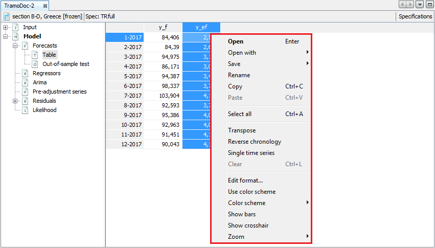
A local menu for a selected series in the Table panel

The Out-of-sample test section presents two tests. These tests check the performance of the out-of-sample forecasts, by comparison of forecast limits and the data. To perform this exercise, first the historical data sample is divided into a fit period (whole estimation span excluding last 18 observations) and a test period (last 18 observations). For the fit period the model is automatically selected and its parameters are fixed. The model is used to produce a one-period-ahead forecast (i.e. the forecast for $\mathbf{n + 1}$, where $\mathbf{n}$ is the length of the time series). This estimation is performed 18 times for the gradually extended time series.

The first test compares forecast errors with the standard error of the in-sample residuals. The goodness of fit is assessed by checking if the mean of the forecast errors can be assumed zero.

The second test compares mean squared of forecast error with mean squared of in-sample residuals. The result of the test is accepted when these two indicators are close to each other. The lack of consistency is a clear evidence of a model inadequacy.

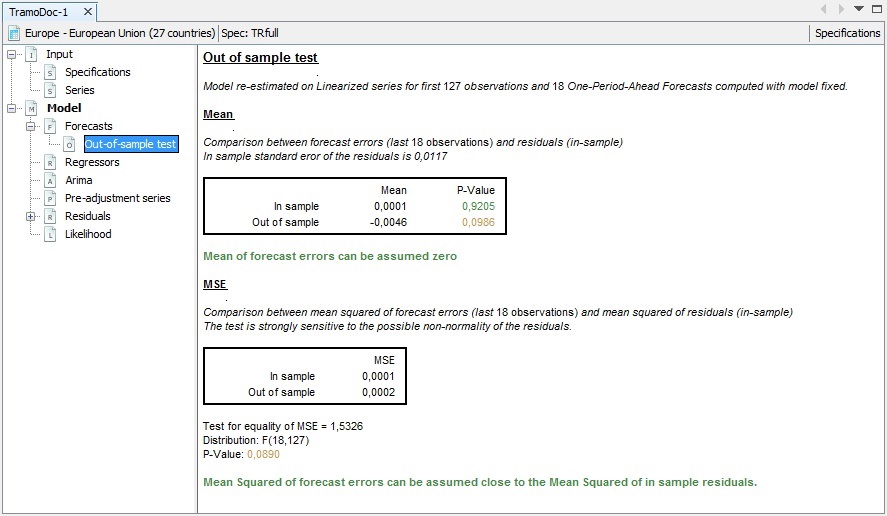
An example of out-of-sample test results