Output from the X13 procedure
The X-13ARIMA-SEATS method consists of two linked parts: the RegARIMA model and the decomposition step that can be performed using the X-11 algorithm or the SEATS program. The results from the RegARIMA model, which are displayed under the Output from a modelling procedure section. The output from the decomposition step is presented in the three nodes: Decomposition, Benchmarking and Diagnostics. The majority of indicators displayed in the Diagnostics are shared with TRAMO-SEATS. For the Main results node only one section is different from the output produced by TRAMO-SEATS. This section focuses on the nodes that are not handled elsewhere, i.e. the output produced by X-11. Therefore the sections that are explained here are Decomposition and some parts of the Main results and Diagnostics sections. Their content is accessible once the user selects the appropriate node from the left-hand side seasonal adjustment results panel.
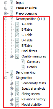
The structure of the results for X-13ARIMA-SEATS
Main results
The first section of the Main results node summarises the results of the pre-processing. The content of this panel depends on the specifications used for processing and the results of the seasonal adjustment1. In the case of the pre-defined specifications X11, RSA0, RSA1 and RSA3 no trading day effect is estimated. For RSA2c and RSA4c pre-defined specifications, working day effects and the leap year effect are pre-tested and estimated if present. If the working day effect is significant, the pre-processing part includes the message Working days effects (1 variable). The message Working days effects (2 variables) means that the leap year effect has also been estimated. For RSA5c the trading day effect and the leap year effect are pre-tested. If the trading day effect has been detected, either of the messages Trading days effects (6 variables) or Trading days effects (7 variables) are displayed, depending whether the leap year effect has been detected or not. If the Easter effect is statistically significant, Easter effect detected is displayed. In this section, only the total number of detected outliers is visible. More detailed information on each outlier, i.e. type, location and estimated coefficient, can be found in the Pre-processing node.
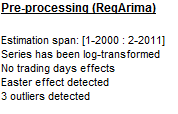
The summary of the results from RegARIMA
The message Series has been log-transformed is only displayed if a logarithmic transformation has been applied. Otherwise, the message does not appear.
The m-statistics section provides summary indicators (\(q\) and \(q - m2)\ \)from analysis of M-statistics. The result displayed in green indicates that the given indicator’s value has been accepted. When the indicator is above one, the test fails and the statistic is displayed in red.
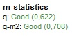
The summary of m-statistics
Decomposition (X11)
This part includes tables with results from consecutive iterations of the X-11 algorithm and the set of quality measures.
Tables
The decomposition step of X-13ARIMA-SEATS is performed by an iterative algorithm X-11, which general principle is an estimation of the different components using the appropriate moving averages. The results of each step of the algorithm are saved in the successive tables, which are displayed in this section. However, some tables produced by the original X-11 algorithm are omitted. The tables are divided into six groups, which correspond to the main steps of the algorithm:
-
Part A: Pre-adjustments;
-
Part B: First automatic correction of the series;
-
Part C: Second automatic correction of the series;
-
Part D: Seasonal adjustment;
-
Part E: Components modified for large extreme values;
-
Part F: Seasonal adjustment quality measures.
As an example the view of the D-table group is presented below.
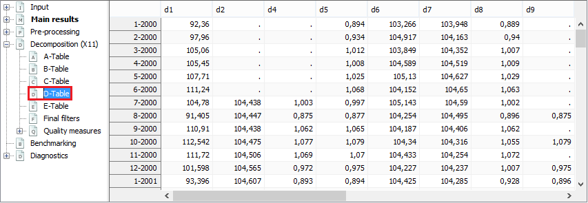
The outcome of the part D of the X-11 algorithm
By default, each table is displayed as a time series. To switch into table view select the Single time series option from the local menu.
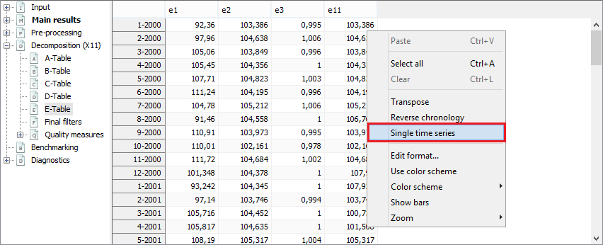
The local menu for the X-11 tables
Then, to display a given table expand the menu, which is available above the table, and choose table’s name.
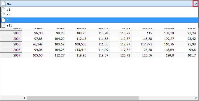
X-11 outcomes presented as tables
Final filters
The length of the seasonal and trend moving average filters used to estimate the final seasonal factors and the final trend depend on the time series and are selected automatically by the X-11 algorithm on a basis of the time series properties. In short, JDemetra+ selects the filters automatically, taking into account the global moving seasonality ratio, which is computed on preliminary estimates of the irregular component and of the seasonal. In the case of user-defined seasonal adjustment specifications, the lengths of the seasonal and trend filters can be chosen manually.
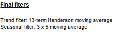
Information about filters used by the X-11 algorithm to calculate the final estimate of the seasonal component and trend
For user-defined specifications the different seasonal filters can be applied for each period. In such case JDemetra+ informs that the composite filter has been applied. The orders of seasonal filters can be checked in the Specification panel in the X11 → Details on seasonal filter section.
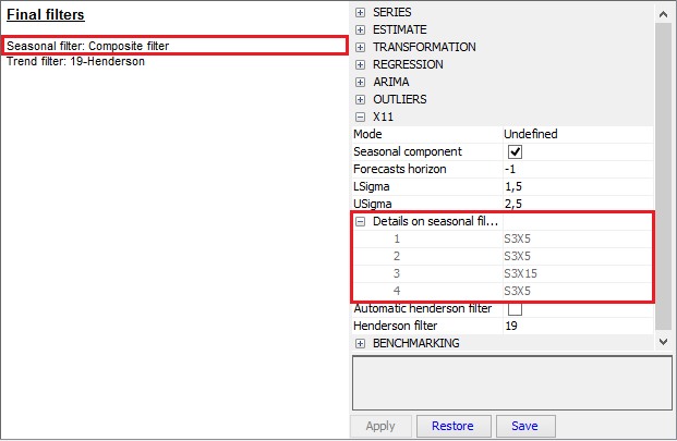
Information about filters used by the X-11 algorithm to calculate the final estimate of the seasonal component and trend – the case of the composite filters
Quality measures
The quality measures are tools that can be used to assess the quality of the decomposition and determine the steps for improvement, if necessary. The set of these measures includes 11 so called \(M\) statistics and two synthetic measures: \(Q\) and \(Q - M2.\)
The \(M\) statistics are used to assess the quality of the seasonal adjustment2. These statistics vary between 0 and 3 but only values smaller than 1 are acceptable. JDemetra+ displays their results together with the composite indicators \(Q\) and \(Q - M2.\) Results displayed in red indicate that the test failed.
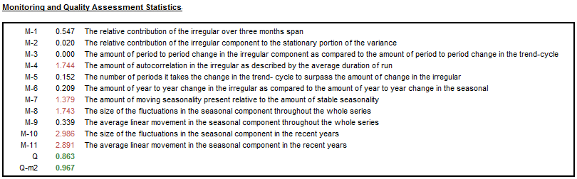
X-11 quality measures
The details about the measures are given below.
-
\(M1\) measures the contribution of the irregular component to the total variance. When it is above 1 some changes in outlier correction should be considered.
-
\(M2\), which is a very similar to \(M1\), is calculated on the basis of the contribution of the irregular component to the stationary portion of the variance. When it is above 1, some changes in an outlier correction should be considered.
-
\(M3\) compares the irregular to the trend taken from a preliminary estimate of the seasonally adjusted series. If this ratio is too large, it is difficult to separate the two components from each other. When it is above 1 some changes in outlier correction should be considered.
-
\(M4\) tests the randomness of the irregular component. A value above 1 denotes a correlation in the irregular component. In such case a shorter seasonal moving average filter should be considered.
-
\(M5\) is used to compare the significance of changes in the trend with that in the irregular. When it is above 1 some changes in outlier correction should be considered.
-
\(M6\) checks the \(\text{SI}\) (seasonal – irregular components ratio). If annual changes in the irregular component are too small in relation to the annual changes in the seasonal component, the \(3 \times 5\) seasonal filter used for the estimation of the seasonal component is not flexible enough to follow the seasonal movement. In such case a longer seasonal moving average filter should be considered. It should be stressed that \(M6\) is calculated only if the \(3 \times 5\) filter has been applied in the model.
-
\(M7\) is the combined test for the presence of an identifiable seasonality. The test compares the relative contribution of stable and moving seasonality3.
-
\(M8\) to \(M11\) measure if the movements due to the short-term quasi-random variations and movements due to the long-term changes are not changing too much over the years. If the changes are too strong then the seasonal factors could be erroneous. In such case a correction for a seasonal break or the change of the seasonal filter should be considered.
The \(Q\) statistic is a composite indicator calculated from the \(M\) statistics.
| \[Q = \frac{10M1 + 11M2 + 10M3 + 8M4 + 11M5 + 10M6 + 18M7 + 7M8 + 7M9 + 4M10 + 4M11}{100}\] | [1] |
\(Q = Q - M2\) (also called \(Q2\)) is the \(Q\) statistic for which the \(M2\) statistics was excluded from the formula, i.e.:
| \[Q - M2 = \frac{10M1 + 10M3 + 8M4 + 11M5 + 10M6 + 18M7 + 7M8 + 7M9 + 4M10 + 4M11}{89}\] | [2] |
If a time series does not cover at least 6 years, the \(M8\), \(M9\), \(M10\) and \(M11\) statistics cannot be calculated. In this case the \(Q\) statistic is computed as:
| \[Q = \frac{14M1 + 15M2 + 10M3 + 8M4 + 11M5 + 10M6 + 32M7}{100}\] | [3] |
The model has a satisfactory quality if the \(Q\) statistic is lower than 1.
The tables displayed in the Quality measures → Details node correspond to the F-set of tables produced by the original X-11 algorithm. To facilitate the analysis of the results, the numbers and the names of the tables are given under each table following the convention used in LADIRAY, D., and QUENNEVILLE, B. (1999).
The first table presents the average percent change without regard to sign of the percent changes (multiplicative model) or average differences (additive model) over several periods (from 1 to 12 for a monthly series, from 1 to 4 for a quarterly series, from 1 to 2 for a half-yearly series) for the following series:
- \(O\) – Original series (Table A1);
-
\(\text{CI}\) – Final seasonally adjusted series (Table D11);
-
\(I\) – Final irregular component (Table D13);
-
\(C\) – Final trend (Table D12);
-
\(S\) – Final seasonal factors (Table D10);
-
\(P\) – Preliminary adjustment coefficients, i.e. regressors estimated by the RegARIMA model (Table A2);
-
\(TD\& H\) – Final calendar component (Tables A6 and A7);
-
\(\text{Mod.O}\) – Original series adjusted for extreme values (Table E1);
-
\(\text{Mod.CI}\) – Final seasonally adjusted series corrected for extreme values (Table E2);
-
\(\text{Mod.I}\) – Final irregular component adjusted for extreme values (Table E3).
In the case of an additive decomposition, for each component the average absolute changes over several periods are calculated as4:
\(\text{Component}_{d} = \frac{1}{n - d}\sum_{t = d + 1}^{n}|Table_{t} - Table_{t - d}|\) [4]
where:
\(d\) – time lag in periods (from a monthly time series \(d\) varies from to 4 or from 1 to 12);
\(n\) – total number of observations per period;
\(\text{Component}\) – the name of the component;
\(\text{Table}\) – the name of the table that corresponds to the component.
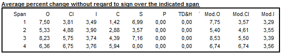
Table F2A – changes, in the absolute values, of the principal components
Next, Table F2B of relative contributions of the different components to the differences (additive model) or percent changes (multiplicative model) in the original series is displayed. They express the relative importance of the changes in each component. Assuming that the components are independent, the following relation is valid:
| \(O_{d}^{2} \approx C_{d}^{2} + S_{d}^{2} + I_{d}^{2} + P_{d}^{2} + {TD\& H}_{d}^{2}\). | [5] |
In order to simplify the analysis, the approximation can be replaced by the following equation:
| \(O_{d}^{*2} = C_{d}^{2} + S_{d}^{2} + I_{d}^{2} + P_{d}^{2} + {TD\& H}_{d}^{2}\). | [6] |
The notation is the same as for Table F2A. The column \(\text{Total}\) denotes total changes in the raw time series.
Data presented in Table F2B indicate the relative contribution of each component to the percent changes (differences) in the original series over each span, and are calculated as:
\(\frac{I_{d}^{2}}{O_{d}^{*2}}\),
\(\frac{C_{d}^{2}}{O_{d}^{*2}}\),
\(\frac{S_{d}^{2}}{O_{d}^{*2}}\),
\(\frac{P_{d}^{2}}{O_{d}^{*2}}\)
and \(\frac{TD\& H_{d}^{2}}{O_{d}^{*2}}\)
where: \(O_{d}^{*2} = I_{d}^{2} + C_{d}^{2} + S_{d}^{2} + P_{d}^{2}{+ TD\& H}_{d}^{2}\).
The last column presents the Ratio calculated as:
\(100 \times \frac{O_{d}^{*2}}{O_{d}^{2}}\),
which is an indicator of how well the approximation
\({(O_{d}^{*})}^{2} \approx O_{d}^{2}\)
holds.
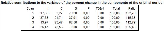
Table F2B – relative contribution of components to changes in the raw series
When an additive decomposition is used, Table F2C presents the average and standard deviation of changes calculated for each time lag \(d\), taking into consideration the sign of the changes of the raw series and its components. In case of a multiplicative decomposition the respective table shows the average percent differences and related standard deviations.
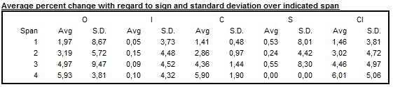
Table F2C – Averages and standard deviations of changes as a function of the time lag
Average duration of run is an average number of consecutive monthly (or quarterly) changes in the same direction (no change is counted as a change in the same direction as the preceding change). JDemetra+ displays this indicator for the seasonally adjusted series, for the trend and for the irregular component.
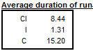
Table F2D – Average duration of run
The \(\frac{I}{C}\ \)ratios for each value of time lag \(d\), presented in Table F2E, are computed on a basis of the data in Table F2A.
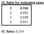
Table F2E – \(\frac{\mathbf{I}}{\mathbf{C}}\mathbf{\ }\)ratio for periods span
The relative contribution of components to the variance of the stationary part of the original series is calculated for the irregular component (\(I\)), trend made stationary5 (\(C\)), seasonal component (\(S\)) and calendar effects (TD&H). The short description of the calculation method is given in LADIRAY, D., and QUENNEVILLE, B. (1999).
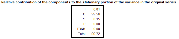
Table F2F – Relative contribution of components to the variance of the stationary part of the original series
The last table shows the autocorrelogram of the irregular component from Table D13. In the case of multiplicative decomposition it is calculated for time lags between 1 and the number of periods per year +2 using the formula6:
\(\text{Corr}_{k}I = \frac{\sum_{t = k + 1}^{N}{(I_{t} - 1)(I_{t - k} - 1)}}{\sum_{t = 1}^{N}{(I_{t} - 1)}^{2}}]\) [7]
where \(N\) is number of observations in the time series and \(\text{k}\) the lag.
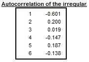
Table F2G – Autocorrelation of the irregular component
The Cochran test is design to identify the heterogeneity of a series of variances. X-13-ARIMA-SEATS uses this test in the extreme value detection procedure to check if the irregular component is heteroskedastic. In this procedure the standard errors of the irregular component are used for an identification of extreme values. If the null hypothesis that for all the periods (months, quarters) the variances of the irregular component are identical is rejected, the standard errors will be computed separately for each period (in case the option Calendarsigma=signif has been selected).
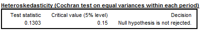
Cochran test
For each \(i^{\text{th}}\) month we will be looking at the mean annual changes for each component by calculating:
\[{\overline{S}}_{i} = \frac{1}{N_{i} - 1}\sum_{t = 2}^{N_{i}}|S_{i,t} - S_{i,t - 1}|\]and
\({\overline{I}}_{i} = \frac{1}{N_{i} - 1}\sum_{t = 2}^{N_{i}}| I_{i,t} - I_{i,t - 1}|\),
where \(N_{i}\) refers to the number of months \(\text{i}\) in the data, and the moving seasonality ratio of month \(i\):
\[MSR_{i} = \frac{\overline{I}_{i}}{\overline{S}_{i}}\]These ratios are published in Table D9A in X13ARIMA-SEATS software. In JDemetra+ they are presented in the details of the quality measures.
The Moving Seasonality Ratio (MSR) is used to measure the amount of noise in the Seasonal-Irregular component. By studying these values, the user can select for each period the seasonal filter that is the most suitable given the noisiness of the series.
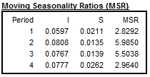
Table D9a – Moving seasonality ratios
-
For description of the pre-defined specifications see sections Seasonal adjustment specifications and Modelling specifications. Also see User-defined specifications section for more detail. ↩
-
For the definitions of the M and Q statistics see LADIRAY, D., and QUENNEVILLE, B. (1999). ↩
-
See section Combined seasonality tests. ↩
-
For the multiplicative decomposition the following formula is used: \(\text{Component}_{d} = \frac{1}{n - d}\sum_{t = d + 1}^{n}{|\frac{\text{Tabl}e_{t}}{\text{Table}_{t - d}} - 1|}\). ↩
-
The component is estimated by extracting a linear trend from the trend component presented in Table D12. ↩
-
For the additive decomposition the formula is: \(Corr_{k}I_{t} = \frac{\sum_{t = k + 1}^{N}{(I_{t} \times I_{t - k})}}{\sum_{t = 1}^{N}{(I_{t})}^{2}}\) ↩