Linearisation with the TRAMO and RegARIMA models

The primary aim of seasonal adjustment is to remove the unobservable seasonal component from the observed series. The decomposition routines implemented in the seasonal adjustment methods make specific assumptions concerning the input series. One of the crucial assumptions is that the input series is stochastic, i.e. it is clean of deterministic effects. Another important limitation derives from the symmetric linear filter used in TRAMO-SEATS and X-13ARIMA-SEATS. A symmetric linear filter cannot be applied to the first and last observations with the same set of weights as for the central observations¹. Therefore, for the most recent observations these filters provide estimates that are subject to revisions.

To overcome these constrains both seasonal adjustment methods discussed here include a modelling step that aims to analyse the time series development and provide a better input for decomposition purposes. The tool that is frequently used for this purpose is the ARIMA model, as discussed by BOX, G.E.P., and JENKINS, G.M. (1970). However, time series are often affected by the outliers, other deterministic effects and missing observations. The presence of these effects is not in line with the ARIMA model assumptions. The presence of outliers and other deterministic effects impede the identification of an optimal ARIMA model due to the important bias in the estimation of parameters of sample autocorrelation functions (both global and partial)². Therefore, the original series need to be corrected for any deterministic effects and missing observations. This process is called linearisation and results in the stochastic series that can be modelled by ARIMA.

For this purpose both TRAMO and RegARIMA use regression models with ARIMA errors. With these models TRAMO and RegARIMA also produce forecasts.

$z_{t} = y_{t}\mathbf{\beta} + x_{t}$, [1]

where:

$z_{t}$ is the original series;

$\mathbf{\beta} = (\beta_{1},\ldots,\beta_{n})$ – a vector of regression coefficients;

$y_{t} = (y_{1t},\ldots,y_{\text{nt}})$ – $\text{n}$ regression variables (the trading day variables, the leap year effect, outliers, the Easter effect, ramps, intervention variables, user-defined variables);

$x_{t}\ $– a disturbance that follows the general ARIMA process: $\phi\left( B \right)\delta\left( B \right)x_{t} = \theta(B)a_{t}$; $\phi\left( B \right)$,$\ \theta(B)$ and $\delta\left( B \right)$ are the finite polynomials in $B$; $a_{t}$ is a white-noise variable with zero mean and a constant variance.

The polynomial $\phi\left( B \right)$ is a stationary autoregressive (AR) polynomial in $B$, which is a product of the stationary regular AR polynomial in $B$ and the stationary seasonal polynomial in $\text{B}^{s}$:³

\(\phi\left( B \right) = \phi_{p}\left( B \right)\Phi_{p_{s}}\left( B^{s} \right) = (1 + \phi_{1}B + \ldots + \phi_{p}B^{p})(1 + \Phi_{1}B^{s} + \ldots + \Phi_{p_{s}}B^{p_{s}s})\) [2]

where:

$\text{p}$ – the number of regular AR terms, (in JDemetra+$\ \ p \leq 3)$;

$p_{s}$ – the number of seasonal AR terms, (in JDemetra+ $p_{s} \leq 1)$;

$\text{s}$ – the number of observations per year (frequency of the time series).

The polynomial $\theta(B)$ is an invertible moving average (MA) polynomial in $B$, which is a product of the invertible regular MA polynomial in $B$ and the invertible seasonal MA polynomial in $\text{B}$:

$\theta\left( B \right) = \theta_{q}\left( B \right)\Theta_{q_{s}}\left( B^{s} \right) = (1 + \theta_{1}B + \ldots + \theta_{q}B^{q})(1 + \Theta_{1}B^{s} + \ldots + \Theta_{q_{s}}B^{q_{s}s})$, [3]

where:

$q$ – the number of regular MA terms, ($q \leq 3)$;

$q_{s}$ – the number of seasonal MA terms, ($q_{s} \leq 1)$.

An MA polynomial (1+$\theta_{1}B + \ldots + \theta_{q}B^{q})\ $is invertible if all its roots lie outside the unit circle, i.e. their modulus is greater than 1. When invertible an MA process, $x_{t} = \theta\left( B \right)a_{t},$ can be expressed as

An AR process of infinite order, $\pi\left( B \right)x_{t} = a_{t}$, where , $\pi\left( B \right) = \pi_{0} + \pi_{1}B + \ldots$ ⁴

The polynomial $\delta\left( B \right)$ is the non-stationary AR polynomial in $B$ (unit roots):

$\delta\left( B \right) = {(1 - B)}^{d}{(1 - B^{s})}^{d_{s}}$, [4]

where:

$d$ – regular differencing order, ($d \leq 1)$;

$d_{s}\ $– seasonal differencing order, ($d_{s} \leq 1)$.

JDemetra+ uses notation: $P,\ D,\ Q,BP,\ BD,\ BQ$ instead of, respectively:$\ p,\ d,q,p_{s},\ d_{s},\ q_{s}$. Therefore, the structure of the ARIMA$\ (p,\ d,\ q)(P,\ D,\ Q)$ model is denoted in JDemetra+ as ARIMA $(P,\ D,\ Q)(BP,\ BD,\ BQ)$.

Both TRAMO and X-12-ARIMA allows for an automatic identification of an ARIMA model extended for the regression variables. The procedure includes a test for logarithmic transformation (so-called the test for the log-level specification), selection of the ARIMA model structure and regressors. The estimated deterministic effects are removed from the time series to improve the estimation of the time series components. Forecasts produced by the ARIMA model provide an input for the linear filters used in the decomposition step. In summary, the application of an ARIMA model to the original series vastly improves the quality and stability of the estimated components. The details of the estimation procedure of the ARIMA model with regression variables are presented in the later in this section.

Among the deterministic effects one can distinguish between the calendar effects and outliers. The calendar effects are discussed in the Calendar effects section. The impact of different types of outliers on time series is illustrated with several examples by FRANSES, P.H. (1998) For example, it was explained that additive outliers, which are described later in this section, yield large values of skewness and kurtosis, and hence failure of a normality test. They also increase the standard error of the estimation parameters. This effect is especially prominent when the size of the outlier is considerable.

KAISER, R., and MARAVALL, A. (1999) express the impact of the outliers on the observed series as:⁵

$y_{t}^{*} = \sum_{j = 1}^{k}\xi_{j}\left( B \right)\omega_{j}I_{t}^{\left( \tau_{j} \right)} + y_{t}$, [5]

where:

$y_{t}^{*}$ – an observed time series;

$y_{t}$ – a series that follows the ARIMA model;

$\omega_{j}$ – an initial impact of the outlier at time ${t = \tau}_{j}$;

$I_{t}^{\left( \tau_{j} \right)}$ – an indicator variable such that is 1 for ${t = \tau}_{j}$ and 0 otherwise;

$\xi_{j}\left( B \right)$ – an expression that determines the dynamics of the outlier occurring at time ${t = \tau}_{j}$;

$B$ – a backshift operator (i.e. $B^{k}X_{t} = X_{t - k}$).

The optimal choice of regression variables (and/or intervention variables) requires knowledge from the user about the time series being modelled⁶. On the contrary, outliers, frequently used in modelling seasonal economic time series, can be automatically detected by JDemetra+ (see Specifiations - TRAMO section for TRAMO and Specifiations - ARIMA section for RegARIMA). The procedure described in GÓMEZ, V., and MARAVALL, A. (2001a) identifies the ARIMA model structure in the presence of deterministic effects. Therefore, the number of identified outliers may depend on the ARIMA model estimated on the series.

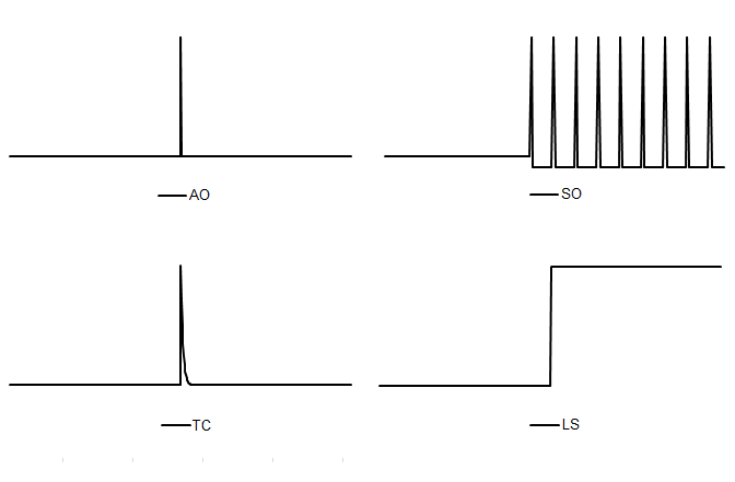
The types of outliers that can be automatically identified and estimated by JDemetra+ without any user intervention are:

• Additive Outlier (AO) – a point outlier which occurs at a given time $t_0$. For the additive outlier $\xi_{j}( B) = 1$, which results in the regression variable:

\(AO_{t}^{t_{0}} = \begin{cases} 1 \text{ for } t = t_{0} \\\\ 0 \text{ for } t \neq t_{0} \end{cases}\); [6]

• Level shift (LS) – a variable for a constant level shift beginning at the given time $t_{0}$. For the level shift $\xi_{j}\left( B \right) = \frac{1}{1 - B}$, which results in the regression variable:

\(LS_{t}^{t_{0}} = \begin{cases} -1 \text{ for } t < t_{0} \\\\ 0 \text{ for } t \geq t_{0} \end{cases}\); [7]

• Temporary change⁷ (TC) – a variable for an effect on the given time $t_{0}$ that decays exponentially over the following periods. For the temporary change $\xi_{j}\left( B \right) = \frac{1}{1 - \delta B}$, which results in the regression variable:

\(TC_{t}^{t_{0}} = \begin{cases} 0 \text{ for } t < t_{0} \\\\ \alpha^{t - t_{0}} \text{ for } t \geq t_{0} \end{cases}\); [8]

where $\alpha$ is a rate of decay back to the previous level $(0 < \alpha < 1)$.

• Seasonal outliers (SO) – a variable that captures an abrupt change in the seasonal pattern on the given date $t_{0}\ $and maintains the level of the series with a contrasting change spread over the remaining periods. It is modelled by the regression variable:

\(SO_{t}^{t_{0}} = \begin{cases} 0 \text{ for } t < t_{0} \\\\ 1 \text{ for } t \geq t_{0}, \text{$t$ same month/quarter as $t_{0}$} \\\\ \frac{- 1}{(s - 1)} \text{ otherwise} \end{cases}\); [9]

where $s$ is a frequency of the time series ($s = 12\ $for a monthly time series, $s = 4\ $for a quarterly time series).

The shapes generated by the formulas given above are presented in the figure below.

Pre-defined outliers built in to JDemetra+

Within the RegARIMA model it can be also tested if a series of level shifts cancels out to form a temporary level change effect, which is a permanent level shift spanned between two given dates. It is modelled by the regression variable:

\(TLS_{t}^{ {(t}_{0}{,\ t}_{1})} = \begin{cases} 0 \text{ for } t < t_{0} \\\\ 1 \text{ for } t_{1} \geq t \geq t_{0} \\\\ 0 \text{ for } t > t_{1} \end{cases}\); [10]

JDemetra+ also identifies other pre-defined regression variables, for which a necessary input, such as location and process that generates the variable, is provided by the user. This group includes:

• Ramp – a variable for a linear increase or decrease in the level of the series over a specified time interval $t_{0}$ to$\ t_{1}$. It is modelled by a regression variable:

\(RP_{t}^{ {(t}_{0}{,\ t}_{1})} = \begin{cases} -1 \text{ for } t \leq t_{0} \\\\ -\frac{t - t_{0}}{t_{1} - t_{0}} - 1 \text{ for } t_{0} < t < t_{1} \\\\ 0 \text{ for } t \geq t_{1} \end{cases}\); [11]

Intervention variables which are combinations of five basic structures⁸:

• dummy variables⁹;

• any possible sequence of ones and zeros;

• $\frac{1}{(1 - \delta B)}$, $(0 < \delta \leq 1)$;

• $\frac{1}{(1 - \delta_{s}B^{s})}$, $(0 < \delta_{s} \leq 1)$;

• $\frac{1}{(1 - B)(1 - B^{s})}$;

where $s$ is frequency of the time series ($s = 12\ $for a monthly time series, $s = 4\ $for a quarterly time series).

The structures considered by intervention variables allow for generation of all pre-defined outliers described by [6] – [11], as well as some more sophisticated effects. An example can be a level shift effect reached after a sequence of damped overshootings and undershootings, presented in the figure below and denoted there as IV. Another example of an outlier that can be created with intervention variables is a pure seasonal outlier ($PSO)$, which, in contrast to the seasonal outlier described above, does not affect the trend. The set of pure seasonal outliers is used to model the seasonal change of regime ($\text{SCR}$) effect, which describes a sudden and sustained change in the seasonal pattern affecting from $t_{0}$ (possibly) all seasons of the series. It is defined as:

\(SCR_{i,j} = \begin{cases} 1 \text{ for } t \epsilon j \text{ and } t < t_{0} \\\\ 0 \text{ for } t \notin j \text{ or } t \geq t_{0} \\\\ -1 \text{ for } t \epsilon s \text{ and } t < t_{0} \end{cases}\); [12]

where $j = 1,\ldots s - 1$.

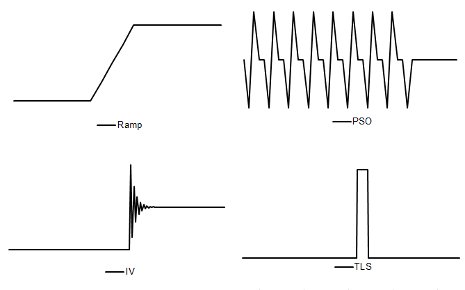
Examples of intervention variables

Automatic model identification procedure in TRAMO

An algorithm for Automatic Model Identification in the Presence of Outliers (AMI) implemented in TRAMO is based on TSAY, C. (1986) and CHEN, B.-C., and LIU, L.-M. (1993) with some modifications (see GÓMEZ, V., and MARAVALL, A. (2001)). It iterates between two stages: the first is automatic outlier detection and correction and the second automatic model identification. The parameters of the AMI procedure are described in the Specifiations - ARIMA section. Unless the parameters are set by the user the program runs with the default values.

The algorithm starts with the identification of the default model and pre-testing procedure, where on the first step a test for a log-level specification is performed. It is based on the maximum likelihood estimation of the parameter $\lambda$ in the Box-Cox transformation, which is a power transformation such that the transformed values of the time series $y\ $are a monotonic function of the observations, i.e. \(y^{\alpha} = \begin{cases} \frac{\left( y_{i}^{\alpha} - 1 \right)}{\lambda}, \lambda \neq 0 \\\\ \log{y_{i}^{\alpha}, \lambda = 0} \end{cases}\);

First, two Airline models (i.e. ARIMA(0,1,1)(0,1,1)) with a mean) are fitted to the time series: one in logs ($\lambda = 0$), other without logs ($\lambda = 1$). The test compares the sum of squares of the model without logs with the sum of squares multiplied by the square of the geometric mean of the (regularly and seasonally) differenced series in the case of the model in logs. Logs are taken in the case this last function is the minimum¹⁰. By default, both TRAMO and X-12-ARIMA have a slight bias towards the log transformation.

Next, the test for calendar effects is performed with regressions using the default model for the noise and, if the model is subsequently changed, the test is redone. For seasonal series the default model is the Airline model (ARIMA (0,1,1)(0,1,1)) while for the non-seasonal series ARIMA (0,1,1)(0,0,0) with a constant term is used. The default model, which is used as a benchmark model at some next steps of AMI, is determined by the result of the pre-test for possible presence of seasonality.

Once these pre-tests have been completed, the original series is corrected for all pre-specified outliers and regression effects provided by the user, if any. Next, the order of the differencing polynomial $\text{δ}\left( B \right)$­ that contains the unit roots is identified and it is decided whether to specify a mean for the series or not. The identification of the ARMA model, i.e. the order of $\phi\left( B \right)\ $and $\text{θ}\left( B \right)\ $ ­is performed using the Hannan and Rissanen method by the means of minimising the Bayesian information criterion with some constraints aimed at increasing the parsimony and favouring balanced models¹¹. This procedure produces the initial values of the ARIMA model parameters. The search is done sequentially: for the fixed regular polynomials, the seasonal ones are obtained, and vice versa. When the estimated roots of the AR and MA processes are close to each other, the order of the ARIMA model can be reduced. The identification and estimation of the model is carried out using Exact Maximum Likelihood (EML) or the Unconditional Least Squares method.

If the calendar effects were identified in the default model, they are included in a new ARIMA model provided that these effects are significant for this model. The estimated residuals from the modified ARIMA model with fixed parameters and the median absolute deviation of the standard deviation of these residuals are used in the outlier detection procedure. For each observation, $t$-tests are computed for all types of outlier considered in the automatic procedure (AO, TC, LS, SO), following the procedure proposed in CHEN, B.-C., and LIU, L.-M. (1993). The program compares$\text{t}$-statistics to a critical value determined by the series length. If there are outliers, for which the absolute $t$-values are greater than a critical value, the one with the greatest absolute$\text{t}$-value is selected. After correcting for the identified outlier, the process is started again to test if there is another outlier. The procedure is repeated until for none of the potential outliers, the $t$-statistic exceeds the critical value. If outliers are detected, then a multiple regression is performed using the Kalman filter and the QR algorithm to avoid (as much as possible) masking effects (i.e. detecting spurious outliers) and to correct for the bias produced in the estimators sequentially obtained². If there are outliers for which the absolute $t$-values are greater than the critical value, the one with the greatest absolute $t$-value is selected and the algorithm continues to the estimation of the ARMA model parameters. Otherwise, the algorithm stops¹². The estimated residuals from the final ARIMA model are checked for adequacy against the estimated residuals produced by the balanced model. The final model identified by the AMI procedure must show some improvement over the default model in these residual diagnostics; otherwise, the program will accept the default model⁶.

Automatic model identification procedure in RegARIMA

The original RegARIMA algorithm developed by the U.S. Census Bureau includes two automatic model selection procedures: automdl that is based on TRAMO and pickmdl that originates from X-11-ARIMA¹³. The algorithm implementation in JDemetra+ for RegARIMA follows the TRAMO logic. It is very similar to the TRAMO procedure presented in the previous section, but contains modifications to make use of the X-13ARIMA-SEATS estimation procedure, which is different from the one that TRAMO uses⁶. The examples of extensions that are specific to RegARIMA only are: special treatment of the leap year effect in the multiplicative model, automatic detection of the length of the Easter effect¹⁴, option to reduce a series of level shifts to the temporary level shift. In comparison with TRAMO, there are also differences in the values of the default parameters. Besides, by default, RegARIMA does not favour balanced models. The log/level test in RegARIMA is based on the Corrected Akaike Information Criterion (AICC). Similarly, the estimation of calendar effects is based on AICC. As a result, the model selected by RegARIMA can differ from the model that TRAMO would select, especially in the case of series contaminated with some deterministic effects and/or those, which are modelled with the mixed ARIMA models.

Model selection criteria

Model selection criteria are statistical tools for selecting the optimal order of the ARIMA model. The basic idea behind all these criteria is to obtain as much explanatory power (measured by the value of the likelihood function) with only a few parameters. The model selection criteria essentially choose the model with the best fit, as measured by the likelihood function, and it is a subject to a penalty term, to prevent over-fitting that increases with the number of parameters in the model.¹⁵ Some of the most well-known information criteria are: Akaike Information Criterion (AIC)¹⁶, Corrected Akaike Information Criterion (AICC)¹⁷, HQ Information Criterion (HannanQuinn)¹⁸ and Schwarz-Bayes Information Criterion (BIC)¹⁹.

The formulae for the model selection criteria used by JDemetra+ are:

\(AIC_{N} = -2L_{N} + {2n}_{p}\) [13]

\(AICC_{N} = - 2L_{N} + 2n_{p}\left( 1 - \frac{n_{p} + 1}{N} \right)^{- 1}\) [14]

\(HQ_{N} = - 2L_{N} + 2n_{p}\text{ln(ln(N))}\) [15]

\(BIC_{N} = - 2L_{N} + n_{p}\text{logN}\) [16]

where:

$\text{N}$– a number of observations in time series;

$n_{p}$ – a number of estimate parameters;

$L_{N}$ – a loglikelihood function.

For each model selection criteria the model with the smaller value is preferred. As it can be shown that AIC is biased for small samples, it is often replaced by AICC. To choose the ARIMA model parameters the original RegARIMA uses AICC while TRAMO uses BIC with some constraints aimed at increasing the parsimony and favouring balanced models. The automatic model identification methods implemented in JDemetra+ mostly use BIC, however other criteria are used as well. It should be noted that the BIC criterion imposes a greater penalty term than AIC and HQ, so that BIC tends to select simpler models than those chosen by AIC. The difference between both criteria can be huge if $N$ is large²⁰.

Hannan-Rissanen algorithm

The Hannan-Rissanen algorithm²¹ is a penalty function method based on the BIC criterion, where the estimates of the ARMA model parameters are computed by means of a linear regression. The Hannan-Rissanen procedure operates on a stationary transformation of the original series, therefore only AR and MA parameters are being identified.

In the first step, a high-order$\ AR(m)$, where $m > max(p,q)$, model is fitted to the time series $X_{t}$. The maximum order of $p$ and $q$ is given a-priori. In JDemetra+ it is equal to 3 for both $p$ and $q$. The residuals \(\widehat{a}_{k}\) from this model are used to provide estimates of the innovations in the ARMA model $a_{t}$:

\(a_{t} = X_{t} - \sum_{k = 1}^{m}{\widehat{a}_{k}X}_{t - k}\) [17]

In the second step the parameters $p$ and $q$ of the ARMA model are estimated using a least squares linear regression of $X_{t}$ onto $X_{t - 1},\ldots X_{t - p},a_{t - 1},\ldots a_{t - q}$ for a combination of values $p$ and $q$. The first step of the procedure is skipped if the ARMA model fitted in the second step includes only an autoregressive part.

Finally, the Hannan-Rissanen algorithm selects a pair of $p$ and $q$ values for which $BIC_{p,q}$ is the smallest. $BIC_{p,q}$ is defined as:

\(\text{BIC}_{p,q} = \log\left( \sigma_{p,q}^{2} \right) + \frac{\left( p + q \right)\log\left( n - d \right)}{n - d}\) [18]

where:

$\sigma_{p,q}^{2}$ is the maximum likelihood estimator of $\sigma^{2}$;

$n - d\ $is the number of series in the (regularly and/or) seasonally differenced series.

The advantage of the Hannan-Rissanen algorithm is the speed of computation in comparison with an exact likelihood estimation.

Initial values for ARIMA model estimation

By default, the initial parameter value in X-13ARIMA-SEATS is 0.1 for all AR and MA parameters. For the majority of time series this default value seems to be appropriate. Introducing better initial values (as might be obtained, e.g., by first fitting the model using conditional likelihood) could slightly speed up a convergence. Users are allowed to introduce manually initial values for AR and MA parameters that are then used to start the iterative likelihood maximization. This is rarely necessary, and, in general, not recommended. A possible exception to this occurs if the initial estimates that are likely to be extremely accurate are already available, such as when one is re-estimating a model with a small amount of new data added to a time series. However, the main reason for specifying initial parameter values is to deal with convergence problems that may arise in difficult estimation situations⁶.

Cancellation of AR and MA factors

A cancellation issue consists in cancelling some factors on both sides of the ARIMA model. This problem concerns the mixed ARIMA $(p,d,q)(P,D,Q)$ models (i.e. $p > 0\ $and$\ q > 0$, or $P > 0$ and $Q > 0$). For example, a cancellation problem occurs with ARMA (1,1) model, $\left( 1 - \phi B \right)z_{t} = (1 - \theta B)a_{t}$ when $\phi = \theta\ $as then model is simply of the form: $z_{t} = a_{t}$. Such model causes problems with convergence of the nonlinear estimation. For this reason the X-13ARIMA-SEATS and TRAMO-SEATS programs deal with a cancellation problem by computing zeros of the AR and MA polynomials. As the cancellation does not need to be exact, the cancellation limit can be provided by the user⁶.

Least squares estimation by means of the QR decomposition

We consider the regression model:

$y = X\beta + \varepsilon$ [19]

The least squares problem consists in minimizing the quantity $\left| X\beta - y \right|^{2}$.

Provided that the regression variables are independent, it is possible to find an orthogonal matrix $Q$, so that $Q \bullet X = \left( \frac{R}{0} \right)$ where $R$ is upper triangular.

We have now to minimize:

\(\left\| QX\beta - Qy \right\|_{2}^{2} = \left\| \left( \frac{R}{0} \right) \ \beta - Qy \right\|_{2}^{2} = \left\| R\beta - a \right\|_{2}^{2} + \left\| b \right\|_{2}^{2}\) [20]

where $Qy_{0\ldots x - 1} = a$ and $Qy_{x\ldots n - 1} = b$.

The minimum of the previous norm is obtained by setting $\beta = R^{- 1}a$. In that case $\left| R\ \beta - a \right|_{2}^{2} = 0$. The residuals obtained by this procedure are then $b$, as defined above.

It should be noted that the $\text{QR}$ factorization is not unique, and that the final residuals also depend on the order of the regression variables (the columns of $X$).