Residuals
Examination of residuals from a fitted model for signs of model inadequacy is a crucial step of a model validation. Therefore, JDemetra+ produces several residual diagnostics and graphs for a detailed validation of the residuals. They are presented in the Residuals section and its subcategories.
The main panel in this section shows residuals from the TRAMO model in the graph and in the table. The graph can be used for visual examination of the residuals. If the model is adequate, the residuals should not contain any obvious, repetitive pattern.
The local menu, which is available for the graph, offers the copy and export options, including sending the graph to the printer and saving the graph as clipboard or as a file in the PNG format. The Copy series option enables the user to select the series used to produce the graph and export it to the another application.
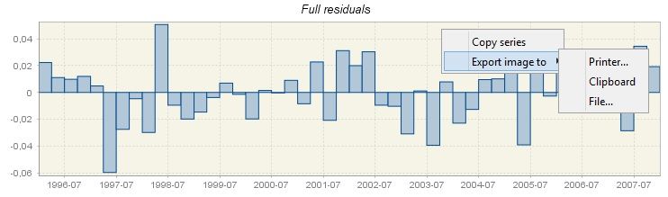
Residuals from the TRAMO model presented in a graph
The lower part of the panel presents the values of the residuals.
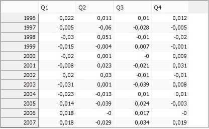
Residuals from the TRAMO model presented in a table
A standard local menu, which is available for this table, includes:
- Select all – copies series and allows it to be pasted into another application e.g. into Excel.
-
Transpose – changes the orientation of the table from horizontal to vertical.
-
Reverse chronology – displays the series from last to first observation
-
Single time series – when it is marked observations are divided by calendar’s periods. Otherwise, data are presented as a standard time series.
-
Edit format – allows changing the format used for displaying dates and values.
-
Use color scheme – allows series values to be displayed in colour.
-
Color scheme – allows for a choice of colour scheme from a pre-specified list.
-
Show bars – presents values in a table as horizontal bars.
-
Zoom – an option for modifying the chart size.
Paste and Clear are disabled as they are not relevant for this view.
Statistics
The aim of the residuals’ diagnostic is to check if it can be assumed that the residuals are random, normally distributed and do not contain any structures that can be successfully modelled. JDemetra+ produces various diagnostic statistics using the residuals from the TRAMO model to scrutinize their properties.
For each test the corresponding p-value is reported. A p-value is the probability of obtaining a test statistic at least as extreme as the one that was actually observed. The results are marked in green, yellow or red, depending on the result of statistical test used. Those in green denote that the problematic characteristic has not been detected (e.g. lack of normality of residuals, a significant autocorrelation in residuals). An outcome in yellow denotes the uncertain results. An outcome in red denotes cases where an issue should be addressed. Hence, test statistics will indicate the need to improve the model. Ideally, the model should be improved so that no test statistics indicate uncertainties in the results.
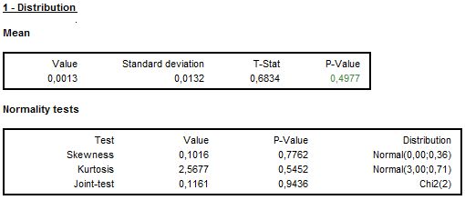
The normality of residuals is crucial for the validity of the prediction intervals produced in forecasting. To assess this property the Doornik-Hansen test is applied. To give more insight into the outcome of this test also the closeness between the residuals mean, skewness and kurtosis is tested. A significant value of one of these statistics indicates that the standardized residuals do not follow a standard normal distribution. The results shown below reveal that the source of uncertain assessment of the normality is a poor skewness performance.
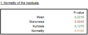
The results of normality of residuals tests
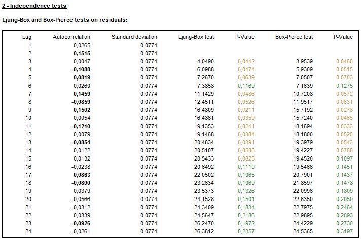
The independence is assessed by the results of the Ljung-Box Q-statistics and the Box-Pierce Q-statistics computed on the regular and seasonal lags. These tests check for the presence of autocorrelation between lags, which is a sign that the values of residuals are not independent. The number of lags that are taken into account depends on the time series frequency. The test on regular lags examines the first 24 lags (for monthly series), the first 16 lags (for quarterly series) or the first 8 lags (half-yearly series). The tests for residual seasonal autocorrelation in residuals consider the first two seasonal lags, irrespective of the time series frequency.
Another test that checks for the presence of autocorrelation in the residuals is the Durbin–Watson statistic. A test outcome that is close to 2 indicates no sign of autocorrelation.
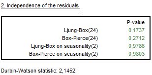
The results of independence of tests on residuals
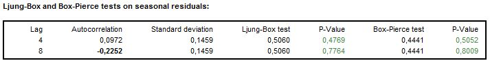
The randomness in the signs of residuals is assessed by the Wald-Wolfowitz test, also called the Run test. It examines the hypothesis that a series of numbers is random. For data centred around the mean, the test calculates the number and length of runs. A run is defined as a set of sequential values that are either all above or all below the mean. An up run is a sequence of numbers each of which is above the mean; a down run is a sequence of numbers each of which is below the mean.
The test checks if the up and down runs are distributed equally in time. Both too many runs and too few runs are unlikely to be a real random sequence. The null hypothesis is that the values of the series have been independently drawn from the same distribution. The test also verifies the hypothesis that the length of runs is random.
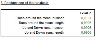
The results of randomness of residuals tests
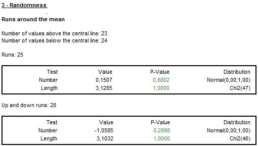
The significant values of the Ljung-Box Q-statistics (or the Box-Pierce Q-statistics) of the squared residuals indicate the random variation of the coefficients or time-varying conditional variances. These effects cannot be modelled by the TRAMO model. Their presences cause the test statistics and forecast coverage intervals to have reduced reliability. The autocorrelation is checked by JDemetra+ for the first 24 lags (monthly series), the first 16 lags (quarterly series) or the first 8 lags (half-yearly series).
The example below shows the p-values marked in red, which indicate that the null hypothesis (no autocorrelation) has been rejected. The outcome of the linearity of the residuals test provides evidence of autocorrelation in residuals, which means that the linear structure is left in the residuals.
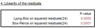
The results of linearity of residuals tests
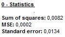
The basic residuals’ characteristics are given in table 0-Statistcs. They include a sum of squares, a mean squared error (MSE) and a standard error of residuals.
Details of residuals basic characteristics
Next section presents the detailed statistics and tests of the distribution of residuals.
The detailed results of normality of residuals tests
To assess the independence in detail, the autocorrelation function of residuals with standard deviations, the Ljung-Box Q-statistics and the Box-Pierce statistics are computed through each lag.
The detailed results of independence of residuals tests
The presence of the autocorrelation at seasonal lags is checked by the Ljung-Box Q-statistics and the Box-Pierce Q-statistics and the respective p-values. They are accompanied by the autocorrelation function of residuals and its standard deviations.
The detailed results of independence of squared residuals tests
The detailed results on various versions of the Run test are given in the next section of the output tree.
The detailed results of randomness of residuals tests
Finally, the autocorrelation function of squared residuals with standard errors, the Ljung-Box Q-statistics and the Box-Pierce Q-statistics computed through each lag can be inspected to assess the presence of residual autocorrelation structures.
The detailed results of linearity of residuals tests
Distribution
The sample autocorrelation function (ACF) and sample partial autocorrelation function (PACF) of the (regularly and seasonally differenced, if necessary) time series \(y_{t}\) are tools used in a well-established procedure of an identification of an ARIMA model that originates from the Box-Jenkins method. The significant lags observed for those functions are signs of an autocorrelation or a moving average processes present in the data. For an identification of the TRAMO models a modified approach is needed, as described in BELL, W.R., and HILLMER, S.C. (1984), since the presence of regression effects can distort the appearance of the ACF and PACF.
As model residuals are expected to be a random process, the ACF and PACF functions for residuals are expected not to contain any significant values. The user is expected to examine these functions in the usual way (check if the significant lags are present).
The ACF and PACF graphs are accompanied by the picture that shows the histogram of the residuals, which is compared with a normal distribution. It is expected that the residuals follow the normal distribution and therefore the consecutive histogram values should be close to the relevant values of the normal distribution plot. The significant lags, however, indicate the presence of an autocorrelation structure left in the residuals.
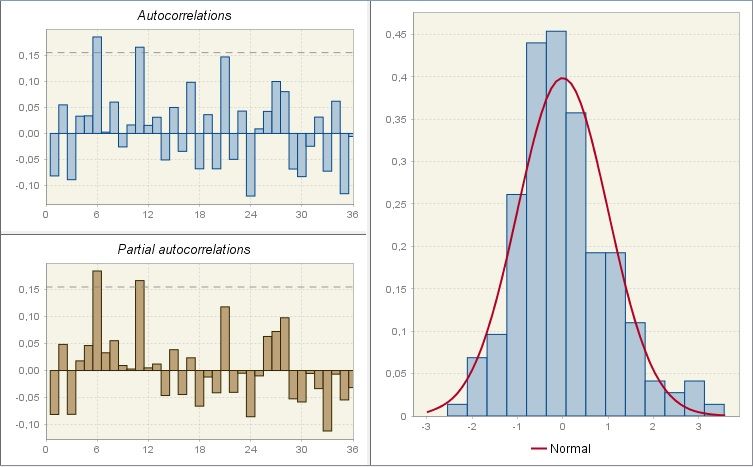
The sample autocorrelation function, sample partial autocorrelation function and distribution of residuals
Spectral analysis
In this section two spectral plots obtained for the residuals from the TRAMO model are displayed. These graphs present two spectrum estimators of the residuals: periodogram and autoregressive spectrum1. They help to reveal any seasonal and trading day effects remaining in the residuals (see also a scenerio that concerns these graphs).
-
The theoretical motivation for the choice of spectral estimator is provided by SOKUP, R., and FINDLEY, D. (1999). ↩