X-11
A complete documentation of the X-11 method is available in LADIRAY, D., and QUENNEVILLE, B. (2001). The X-11 program is the result of a long tradition of non-parametric smoothing based on moving averages, which are weighted averages of a moving span of a time series (see hereafter). Moving averages have two important drawbacks:
-
They are not resistant and might be deeply impacted by outliers;
-
The smoothing of the ends of the series cannot be done except with asymmetric moving averages which introduce phase-shifts and delays in the detection of turning points.
These drawbacks adversely affect the X-11 output and stimulate the development of this method. To overcome these flaws first the series are modelled with a RegARIMA model that calculates forecasts and estimates the regression effects. Therefore, the seasonal adjustment process is divided into two parts.
- In a first step, the RegARIMA model is used to clean the series from
non-linearities, mainly outliers and calendar effects. A global ARIMA model is adjusted to the series in order to compute the forecasts.
- In a second step, an enhanced version of the X-11 algorithm is used
to compute the trend, the seasonal component and the irregular component.
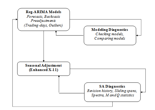
The flow diagram for seasonal adjustment with X-13ARIMA-SEATS using the X-11 algorithm.
Moving averages
The moving average of coefficient $\theta_{i}$ is defined as:
\(M\left( X_{t} \right) = \sum_{k = - p}^{+ f}\theta_{k}X_{t + k}\) [1]
The value at time $t$ of the series is therefore replaced by a weighted average of $p$ "past" values of the series, the current value, and $f$ "future" values of the series. The quantity $p + f + 1\ $is called the moving average order. When $p$ is equal to $f$, that is, when the number of points in the past is the same as the number of points in the future, the moving average is said to be centred. If, in addition, $\theta_{- k} = \theta_{k}$ for any $k$, the moving average $M$ is said to be symmetric. One of the simplest moving averages is the symmetric moving average of order $P = 2p + 1$ where all the weights are equal to$\ \frac{1}{P}$.
This moving average formula works well for all time series observations, except for the first $p$ values and last $f$ values. Generally, with a moving average of order $p + f + 1\ $calculated for instant $t$nwith points $p$ in the past and points $f$ in the future, it will be impossible to smooth out the first $p$ values and the last $f$ values of the series because of lack of input to the moving average formula.
In the X-11 method, symmetric moving averages play an important role as they do not introduce any phase-shift in the smoothed series. But, to avoid losing information at the series ends, they are either supplemented by ad hoc asymmetric moving averages or applied on the series extended by forecasts.
For the estimation of the seasonal component, X-13ARIMA-SEATS uses $P \times Q$ composite moving averages, obtained by composing a simple moving average of order $P$, which coefficients are all equal to $\frac{1}{P}$, and a simple moving average of order $Q$, which coefficients are all equal to $\frac{1}{Q}$.
The composite moving averages are widely used by the X-11 method. For an initial estimation of trend X-11 method uses a $2 \times 4$ moving average in case of a quarterly time series while for a monthly time series a $2 \times 12\ $moving average is applied. The $2 \times 4$ moving average is an average of order 5 with coefficients \(\frac{1}{8}\left\{1, 2, 2, 2, 1\right\}\). It eliminates frequency $\frac{\pi}{2}$ corresponding to period 4 and therefore it is suitable for seasonal adjustment of the quarterly series with a constant seasonality. The $2 \times 12$ moving average, with coefficients \(\frac{1}{24}\left\{1, 2, 2, 2, 2, 2, 2, 2, 2, 2, 2, 2, 1\right\}\)that retains linear trends, eliminates order-$12$ constant seasonality and minimises the variance of the irregular component. The $2 \times 4$ and $2 \times 12$ moving averages are also used in the X-11 method to normalise the seasonal factors. The composite moving averages are also used to extract the seasonal component. These, which are used in the purely automatic run of the X-11 method (without any intervention from the user) are $3 \times 3$, $3 \times 5$ and $3 \times 9$.
In the estimation of the trend also Henderson moving averages are used. These filters have been chosen for their smoothing properties. The coefficients of a Henderson moving average of order $2p + 1$ may be calculated using the formula:
$\theta_{i} = \frac{315\left\lbrack \left( n - 1 \right)^{2} - i^{2} \right\rbrack\left\lbrack n^{2} - i^{2} \right\rbrack\left\lbrack \left( n + 1 \right)^{2} - i^{2} \right\rbrack\left\lbrack {3n}^{2} - 16 - 11i^{2} \right\rbrack}{8n\left( n^{2} - 1 \right)\left( {4n}^{2} - 1 \right)\left( {4n}^{2} - 9 \right)\left( 4n^{2} - 25 \right)}$, [2]
where: $n = p + 2$$n = p + 2$.
The basic algorithm of the X-11 method
The X-11 method is based on an iterative principle of estimation of the different components using appropriate moving averages at each step of the algorithm. The successive results are saved in tables. The list of the X-11 tables displayed in JDemetra+ is included at the end of this section.
The basic algorithm of the X-11 method will be presented for a monthly time series $X_{t}$ that is assumed to be decomposable into trend, seasonality and irregular component according to an additive model $X_{t} = TC_{t} + S_{t} + I_{t}$.
A simple seasonal adjustment algorithm can be thought of in eight steps. The steps presented below are designed for the monthly time series. In the algorithm that is run for the quarterly time series the $2 \times 4$ moving average instead of the $2 \times 12$ moving average is used.
Step 1: Estimation of Trend by $\mathbf{2 \times 12}$ moving average:
$TC_{t}^{(1)} = M_{2 \times 12}(X_{t})$ [3]
Step 2: Estimation of the Seasonal-Irregular component:
$\left( S_{t} + I_{t} \right)^{(1)} = X_{t} - \text{TC}_{t}^{(1)}$ [4]
Step 3: Estimation of the Seasonal component by $\mathbf{3 \times 3}$ moving average over each month:
$S_{t}^{(1)} - M_{3 \times 3}\left\lbrack \left( S_{t} + I_{t} \right)^{(1)} \right\rbrack$ [5]
The moving average used here is a $3 \times 3$ moving average over $5$ terms, with coefficients \(\frac{1}{9} \left\{1, 2, 3, 2, 1 \right\}\). The seasonal component is then centred using a $2 \times 12$ moving average.
\(\widetilde{S}_{t}^{(1)} = S_{t}^{(1)} - M_{2 \times 12}\left( S_{t}^{(1)} \right)\) [6]
Step 4: Estimation of the seasonally adjusted series:
\(SA_{t}^{\left( 1 \right)} = \left( \text{TC}_{t} + I_{t} \right)^{(1)} = X_{t} - {\widetilde{S}}_{t}^{(1)}\) [7]
This first estimation of the seasonally adjusted series must, by construction, contain less seasonality. The X-11 method again executes the algorithm presented above, changing the moving averages to take this property into account.
Step 5: Estimation of Trend by 13-term Henderson moving average:
\(TC_{t}^{(2)} = H_{13}\left( \text{SA}_{t}^{\left( 1 \right)} \right)\) [8]
Henderson moving averages, while they do not have special properties in terms of eliminating seasonality (limited or none at this stage), have a very good smoothing power and retain a local polynomial trend of degree $2$ and preserve a local polynomial trend of degree $3$.
Step 6: Estimation of the Seasonal-Irregular component:
\(\left( S_{t} + I_{t} \right)^{(2)} = X_{t} - \text{TC}_{t}^{(2)}\) [9]
Step 7: Estimation of the Seasonal component by $\mathbf{3 \times 5}$ moving average over each month:
\(S_{t}^{(2)} - M_{3 \times 3}\left\lbrack \left( S_{t} + I_{t} \right)^{(2)} \right\rbrack\) [10]
The moving average used here is a $3 \times 5$ moving average over $7$ terms, of coefficients \(\frac{1}{15} \left\{ 1,\ 2,\ 3,\ 3,\ 3,\ 2,\ 1 \right\}\) and retains linear trends. The coefficients are then normalised such that their sum over the whole $12$-month period is approximately cancelled out:
\({ \widetilde{S}}_{t}^{(2)} = S_{t}^{(2)} - M_{2 \times 12}\left( S_{t}^{(2)} \right)\) [11]
Step 8: Estimation of the seasonally adjusted series:
\(SA_{t}^{\left( 2 \right)} = \left(TC_{t} + I_{t} \right)^{(2)} = X_{t} - {\widetilde{S}}_{t}^{(2)}\) [12]
The whole difficulty lies, then, in the choice of the moving averages used for the estimation of the trend in steps $1$ and $5$ on the one hand, and for the estimation of the seasonal component in steps $3$ and $5$. The course of the algorithm in the form that is implemented in JDemetra+ is presented in the figure below. The adjustment for trading day effects, which is present in the original X-11 program, is omitted here, as since calendar correction is performed by the RegARIMA model, JDemetra+ does not perform further adjustment for these effects in the decomposition step.
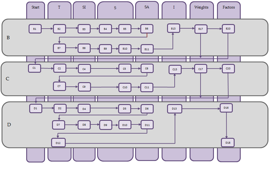
A workflow diagram for the X-11 algorithm based upon training material from the Deutsche Bundesbank
The iterative principle of X-11
To evaluate the different components of a series, while taking into account the possible presence of extreme observations, X-11 will proceed iteratively: estimation of components, search for disruptive effects in the irregular component, estimation of components over a corrected series, search for disruptive effects in the irregular component, and so on.
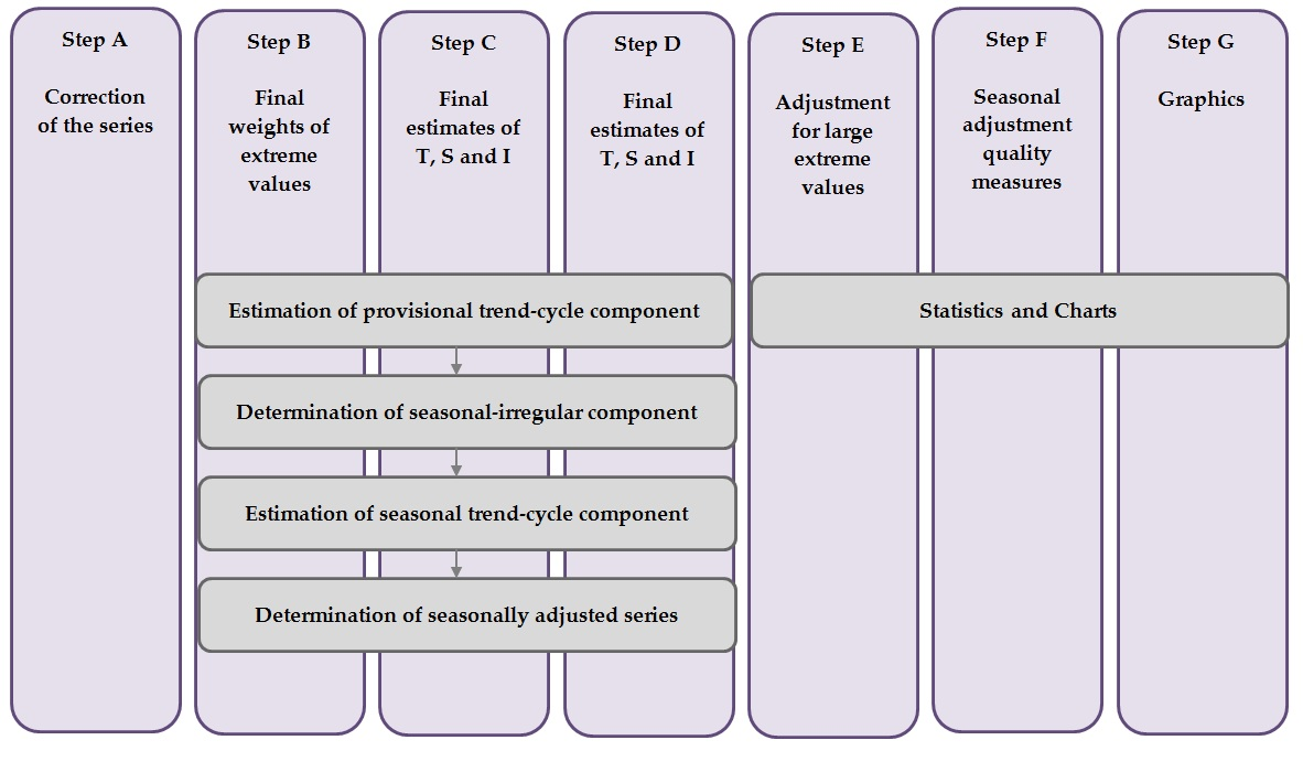
The Census X-11 program presents four processing stages (A, B, C, and D), plus 3 stages, E, F, and G, that propose statistics and charts and are not part of the decomposition per se. In stages B, C and D the basic algorithm is used as is indicated in the figure below.
A workflow diagram for the X-11 algorithm implemented in JDemetra+. Source: Based upon training material from the Deutsche Bundesbank
- Part A: Pre-adjustments
This part, which is not obligatory, corresponds in X-13ARIMA-SEATS to the first cleaning of the series done using the RegARIMA facilities: detection and estimation of outliers and calendar effects (trading day and Easter), forecasts and backcasts1 of the series. Based on these results, the program calculates prior adjustment factors that are applied to the raw series. The series thus corrected, Table B1 of the printouts, then proceeds to part B.
- Part B: First automatic correction of the series
This stage consists of a first estimation and down-weighting of the extreme observations and, if requested, a first estimation of the calendar effects. This stage is performed by applying the basic algorithm detailed earlier. These operations lead to Table B20, adjustment values for extreme observations, used to correct the unadjusted series and result in the series from Table C1.
- Part C: Second automatic correction of the series
Applying the basic algorithm once again, this part leads to a more precise estimation of replacement values of the extreme observations (Table C20). The series, finally "cleaned up", is shown in Table D1 of the printouts.
- Part D: Seasonal adjustment
This part, at which our basic algorithm is applied for the last time, is that of the seasonal adjustment, as it leads to final estimates:
-
of the seasonal component (Table D10);
-
of the seasonally adjusted series (Table D11);
-
of the trend component (Table D12);
-
of the irregular component (Table D13).
- Part E: Components modified for large extreme values
Parts E includes:
-
Components modified for large extreme values;
-
Comparison the annual totals of the raw time series and seasonally adjusted time series;
-
Changes in the final seasonally adjusted series;
-
Changes in the final trend;
-
Robust estimation of the final seasonally adjusted series.
The results from part E are used in part F to calculate the quality measures.
- Part F: Seasonal adjustment quality measures
Part F contains statistics for judging the quality of the seasonal adjustment. JDemetra+ presents selected output for part F, i.e.:
-
M and Q statistics;
-
Tables.
- Part G: Graphics
Part G presents spectra estimated for:
-
Raw time series adjusted a priori (Table B1);
-
Seasonally adjusted time series modified for large extreme values (Table E2);
-
Final irregular component adjusted for large extreme values (Table E3).
Originally, graphics were displayed in character mode. In JDemetra+, these graphics are replaced favourably by the usual graphics software.
The Henderson moving average and the trend estimation
In iteration B (Table B7), iteration C (Table C7) and iteration D (Table D7 and Table D12) the trend component is extracted from an estimate of the seasonally adjusted series using Henderson moving averages. The length of the Henderson filter is chosen automatically by X-13ARIMA-SEATS in a two-step procedure.
It is possible to specify the length of the Henderson moving average to be used. X-13ARIMA-SEATS provides an automatic choice between a 9-term, a 13-term or a 23-term moving average. The automatic choice of the order of the moving average is based on the value of an indicator called $\frac{\overline{I}}{\overline{C}}\ $ratio which compares the magnitude of period-on-period movements in the irregular component with those in the trend. The larger the ratio, the higher the order of the moving average selected. Moreover, X-13ARIMA-SEATS allows the user to choose manually any odd‑numbered Henderson moving average. The procedure used in each part is very similar; the only differences are the number of options available and the treatment of the observations in the both ends of the series. The procedure below is applied for a monthly time series.
In order to calculate $\frac{\overline{I}}{\overline{C}}\ $ ratio a first decomposition of the SA series (seasonally adjusted) is computed using a 13-term Henderson moving average.
For both the trend ($C$) and irregular ($I$) components, the average of the absolute values for monthly growth rates (multiplicative model) or for monthly growth (additive model) are computed. They are denoted as $\overline{C}\ $and $\overline{I}$, receptively, where $\overline{C} = \frac{1}{n - 1}\sum_{t = 2}^{n}\left| C_{t} - C_{t - 1} \right|$ and $\overline{I} = \frac{1}{n - 1}\sum_{t = 2}^{n}\left| I_{t} - I_{t - 1} \right|$.
Then the value of $\frac{\overline{I}}{\overline{C}}\ $ ratio is checked and in iteration B:
-
If the ratio is smaller than 1, a 9-term Henderson moving average is selected;
-
Otherwise, a 13-term Henderson moving average is selected.
Then the trend is computed by applying the selected Henderson filter to the seasonally adjusted series from Table B6. The observations at the beginning and at the end of the time series that cannot be computed by means of symmetric Henderson filters are estimated by ad hoc asymmetric moving averages.
In iterations C and D:
-
If the ratio is smaller than 1, a 9-term Henderson moving average is selected;
-
If the ratio is greater than 3.5, a 23-term Henderson moving average is selected.
-
Otherwise, a 13-term Henderson moving average is selected.
The trend is computed by applying selected Henderson filter to the seasonally adjusted series from Table C6, Table D7 or Table D12, accordingly. At the both ends of the series, where a central Henderson filter cannot be applied, the asymmetric ends weights for the 7 term Henderson filter are used.
Choosing the composite moving averages when estimating the seasonal component
In iteration D, Table D10 shows an estimate of the seasonal factors implemented on the basis of the modified SI (Seasonal – Irregular) factors estimated in Tables D4 and D9bis. This component will have to be smoothed to estimate the seasonal component; depending on the importance of the irregular in the SI component, we will have to use moving averages of varying length as in the estimate of the Trend/Cycle where the $\frac{\overline{I}}{\overline{C}}\ $ ratio was used to select the length of the Henderson moving average. The estimation includes several steps.
Step 1: Estimating the irregular and seasonal components
An estimate of the seasonal component is obtained by smoothing, month by month and therefore column by column, Table D9bis using a simple 7-term moving average, i.e. of coefficients \(\frac{1}{7} \left\{1,\ 1,\ 1,\ 1,\ 1,\ 1,\ 1\right\}\). In order not to lose three points at the beginning and end of each column, all columns are completed as follows. Let us assume that the column that corresponds to the month is composed of $N$ values \(\left\{ x_{1},\ x_{2},\ x_{3},\ \ldots x_{N - 1},\ x_{N} \right\}.\) It will be transformed into a series \(\left\{ {x_{- 2},x_{- 1}{,x}_{0},x}_{1},\ x_{2},\ x_{3},\ \ldots x_{N - 1},\ x_{N},x_{N + 1},\ x_{N + 1},\ x_{N + 2},\ x_{N + 3} \right\}\\) with \(x_{- 2} = x_{- 1} = x_{0} = \frac{x_{1} + x_{2} + x_{3}}{3}\) and \(x_{N + 1} = x_{N + 2} = x_{N + 3} = \frac{x_{N} + x_{N - 1} + x_{N - 2}}{3}\). We then have the required estimates: $S = M_{7}(D9bis)$ and $I = D9bis - S$.
Step 2: Calculating the Moving Seasonality Ratios
For each $i^{\text{th}}$ month the mean annual changes for each component is obtained by calculating \({\overline{S}}_{i} = \frac{1}{N_{i} - 1}\sum_{t = 2}^{N_{i}}\left| S_{i,t} - S_{i,t - 1} \right|\) and \({\overline{I}}_{i} = \frac{1}{N_{i} - 1}\sum_{t = 2}^{N_{i}}\left| I_{i,t} - I_{i,t - 1} \right|\), where $N_{i}$ refers to the number of months $\text{i}$in the data, and the moving seasonality ratio of month $i$: \(MSR_{i} = \frac{\ {\overline{I}}_{i}}{ {\overline{S}}_{i}}\). These ratios are presented in Details of the Quality Measures node under the Decomposition (X11) section. These ratios are used to compare the year-on-year changes in the irregular component with those in the seasonal component. The idea is to obtain, for each month, an indicator capable of selecting the appropriate moving average for the removal of any noise and providing a good estimate of the seasonal factor. The higher the ratio, the more erratic the series, and the greater the order of the moving average should be used. As for the rest, by default the program selects the same moving average for each month, but the user can select different moving averages for each month.
Step 3: Calculating the overall Moving Seasonality Ratio
The overall Moving Seasonality Ratio is calculated as follows:
\(\text{MSR}_{i} = \frac{\sum_{i}^{}{N_{i}\ }\ {\overline{I}}_{i}}{\sum_{i}^{}N_{i}{\overline{S}}_{i}}\) [13]
Step 4: Selecting a moving average and estimating the seasonal component
Depending on the value of the ratio, the program automatically selects a moving average that is applied, column by column (i.e. month by month) to the Seasonal/Irregular component in Table D8 modified, for extreme values, using values in Table D9.
The default selection procedure of a moving average is based on the Moving Seasonality Ratio in the following way:
-
If this ratio occurs within zone A (MSR < 2.5), a $3 \times 3$ moving average is used; if it occurs within zone C (3.5 < MSR < 5.5), a $3 \times 5$ moving average is selected; if it occurs within zone E (MSR > 6.5), a $3 \times 9$ moving average is used;
-
If the MSR occurs within zone B or D, one year of observations is removed from the end of the series, and the MSR is recalculated.
If the ratio again occurs within zones B or D, we start over again, removing a maximum of five years of observations. If this does not work, i.e. if we are again within zones B or D, a $3 \times 5$ moving average is selected.
The chosen symmetric moving average corresponds, as the case may be 5 ($3 \times 3$), 7 $(3 \times 5)\ $or 11 ($3 \times 9$$3 \times 9)$ terms, and therefore does not provide an estimate for the values of seasonal factors in the first 2 (or 3 or 5) and the last 2 (or 3 or 5) years. These are then calculated using associated asymmetric moving averages.
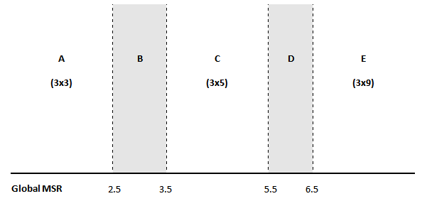
Moving average selection procedure, source: DAGUM, E. B.(1999)
Identification and replacement of extreme values
X-13ARIMA-SEATS detects and removes outliers in the RegARIMA part. However, if there is a seasonal heteroscedasticity in a time series i.e. the variance of the irregular component is different in different calendar months. Examples for this effect could be the weather and snow-dependent output of the construction sector in Germany during winter, or changes in Christmas allowances in Germany and resulting from this a transformation in retail trade turnover before Christmas. The ARIMA model is not on its own able to cope with this characteristic. The practical consequence is given by the detection of additional extreme values by X-11. This may not be appropriate if the seasonal heteroscedasticity is produced by political interventions or other influences. The ARIMA models assume a constant variance and are therefore not by themselves able to cope with this problem. Choosing longer (in the case of diverging weather conditions in the winter time for the construction sector) or shorter filters (in the case of a changing pattern of retail trade turnover in the Christmas time) may be reasonable in such cases. It may even be sensible to take into account the possibility of period-specific (e.g. month-specific) standard deviations, which can be done by changing the default settings of the calendarsigma parameter (see Specifications-X13 section). The value of the calendarsigma parameter will have an impact on the method of calculation of the moving standard deviation in the procedure for extreme values detection presented below.
Step 1: Estimating the seasonal component
The seasonal component is estimated by smoothing the SI component separately for each period using a $3 \times 3$ moving average, i.e.:
\(\frac{1}{9} \times \begin{Bmatrix} 1,0,0,0,0,0,0,0,0,0,0,0, \\ 2,0,0,0,0,0,0,0,0,0,0,0, \\ 3,0,0,0,0,0,0,0,0,0,0,0, \\ 2,0,0,0,0,0,0,0,0,0,0,0, \\ 1,0,0,0,0,0,0,0,0,0,0,0, \\ \end{Bmatrix}\) [14]
Step 2: Normalizing the seasonal factors
The preliminary seasonal factors are normalized in such a way that for one year their average is equal to zero (additive model) or to unity (multiplicative model).
Step 3: Estimating the irregular component
The initial normalized seasonal factors are removed from the Seasonal-Irregular component to provide an estimate of the irregular component.
Step 4: Calculating a moving standard deviation
By default, a moving standard deviation of the irregular component is calculated at five-year intervals. Each standard deviation is associated with the central year used to calculate it. The values in the central year, which in the absolute terms deviate from average by more than the Usigma parameter (by default, 2.5 standard deviations, see Specifications-X13 section) are marked as extreme values and assigned a zero weight. After excluding the extreme values the moving standard deviation is calculated once again.
Step 5: Detecting extreme values and weighting the irregular
The default settings for assigning a weight to each value of irregular component are:
-
Values which are more than Usigma (2.5, by default) standard deviations away (in the absolute terms) from the 0 (additive) or 1 (multiplicative) are assigned a zero weight;
-
Values which are less than 1.5 standard deviations away (in the absolute terms) from the 0 (additive) or 1 (multiplicative) are assigned a full weight (equal to one);
-
Values which lie between 1.5 and 2.5 standard deviations away (in the absolute terms) from the 0 (additive) or 1 (multiplicative) are assigned a weight that varies linearly between 0 and 1 depending on their position.
The default boundaries for the detection of the extreme values can be changed with LSigma and USigma parameters (see Specifications-X13 section).
Step 6: Adjusting extreme values of the seasonal-irregular component
Values of the SI component are considered extreme when a weight less than 1 is assigned to their irregular. Those values are replaced by a weighted average of five values:
-
The value itself with its weight;
-
The two preceding values, for the same period, having a full weight(if available);
-
The next two values, for the same period, having full a weight (if available).
When the four full-weight values are not available, then a simple average of all the values available for the given period is taken.
This general algorithm is used with some modification in parts B and C for detection and replacement of extreme values.
X-11 tables
The list of tables produced by JDemetra+ is presented below. It is not identical to the output produced by the original X-11 program.
Part A – Preliminary Estimation of Outliers and Calendar Effects.
This part includes prior modifications to the original data made in the RegARIMA part:
-
Table A1 – Original series;
-
Table A1a – Forecast of Original Series;
-
Table A2 – Leap year effect;
-
Table A6 – Trading Day effect (1 or 6 variables);
-
Table A7 – The Easter effect;
-
Table A8 – Total Outlier Effect;
-
Table A8i – Additive outlier effect;
-
Table A8t – Level shift effect;
-
Table A8s – Transitory effect;
-
Table A9 – Effect of user-defined regression variables assigned to the seasonally adjusted series or for which the component has not been defined;
-
Table 9sa – Effect of user-defined regression variables assigned to the seasonally adjusted series;
-
Table9u – Effect of user-defined regression variables for which the component has not been defined.
Part B – Preliminary Estimation of the Time Series Components:
-
Table B1 – Original series after adjustment by the RegARIMA model;
-
Table B2 – Unmodified Trend (preliminary estimation using composite moving average);
-
Table B3 – Unmodified Seasonal – Irregular Component (preliminary estimation);
-
Table B4 – Replacement Values for Extreme SI Values;
-
Table B5 – Seasonal Component;
-
Table B6 – Seasonally Adjusted Series;
-
Table B7 – Trend (estimation using Henderson moving average);
-
Table B8 – Unmodified Seasonal – Irregular Component;
-
Table B9 – Replacement Values for Extreme SI Values;
-
Table B10 – Seasonal Component;
-
Table B11 – Seasonally Adjusted Series;
-
Table B13 – Irregular Component;
-
Table B17 – Preliminary Weights for the Irregular;
-
Table B20 – Adjustment Values for Extreme Irregulars.
Part C – Final Estimation of Extreme Values and Calendar Effects:
-
Table C1 – Modified Raw Series;
-
Table C2 – Trend (preliminary estimation using composite moving average);
-
Table C4 – Modified Seasonal – Irregular Component;
-
Table C5 – Seasonal Component;
-
Table C6 – Seasonally Adjusted Series;
-
Table C7 – Trend (estimation using Henderson moving average);
-
Table C9 – Seasonal – Irregular Component;
-
Table C10 – Seasonal Component;
-
Table C11 – Seasonally Adjusted Series;
-
Table C13 – Irregular Component;
-
Table C20 – Adjustment Values for Extreme Irregulars.
Part D – Final Estimation of the Different Components:
-
Table D1 – Modified Raw Series;
-
Table D2 – Trend (preliminary estimation using composite moving average);
-
Table D4 – Modified Seasonal – Irregular Component;
-
Table D5 – Seasonal Component;
-
Table D6 – Seasonally Adjusted Series;
-
Table D7 – Trend (estimation using Henderson moving average);
-
Table D8 – Unmodified Seasonal – Irregular Component;
-
Table D9 – Replacement Values for Extreme SI Values;
-
Table D10 – Final Seasonal Factors;
-
Table D10A – Forecast of Final Seasonal Factors;
-
Table D11 – Final Seasonally Adjusted Series;
-
Table D11A – Forecast of Final Seasonally Adjusted Series;
-
Table D12 – Final Trend (estimation using Henderson moving average);
-
Table D12A – Forecast of Final Trend Component;
-
Table D13 – Final Irregular Component;
-
Table D16 – Seasonal and Calendar Effects;
-
Table D16A – Forecast of Seasonal and Calendar Component;
-
Table D18 – Combined Calendar Effects Factors.
Part E – Components Modified for Large Extreme Values:
-
Table E1 – Raw Series Modified for Large Extreme Values;
-
Table E2 – SA Series Modified for Large Extreme Values;
-
Table E3 – Final Irregular Component Adjusted for Large Extreme Values;
-
Table E11 – Robust Estimation of the Final SA Series.
Part F – Quality indicators:
-
Table F2A – Changes, in the absolute values, of the principal components;
-
Table F2B – Relative contribution of components to changes in the raw series;
-
Table F2C – Averages and standard deviations of changes as a function of the time lag;
-
Table F2D – Average duration of run;
-
Table F2E – I/C ratio for periods span;
-
Table F2F – Relative contribution of components to the variance of the stationary part of the original series;
-
Table F2G – Autocorrelogram of the irregular component.
-
This is a general estimation procedure used by the U.S. Census Bureau. JDemetra+ does not calculate backcasts for X-13ARIMA-SEATS. ↩