Spectral graphs

This scenario is designed for advanced users interested in an in-depth analysis of time series in the frequency domain using three spectral graphs. Those graphs can also be used as a complementary analysis for a better understanding of the results obtained with some of the tests described above.

Economic time series are usually presented in a time domain (X-axis). However, for analytical purposes it is convenient to convert the series to a frequency domain due to the fact that any stationary time series can be expressed as a combination of cosine (or sine) functions. These functions are characterized with different periods (amount of time to complete a full cycle) and amplitudes (maximum/minimum value during the cycle).

The tool used for the analysis of a time series in a frequency domain is called a spectrum. The peaks in the spectrum indicate the presence of cyclical movements with periodicity between two months and one year. A seasonal series should have peaks at the seasonal frequencies. Calendar adjusted data are not expected to have peak at with a calendar frequency.

The periodicity of the phenomenon at frequency f is $\frac{2\pi}{f}$. It means that for a monthly time series the seasonal frequencies $\frac{\pi}{6},\ \frac{\pi}{3},\ \frac{\pi}{2},\ \frac{2\pi}{3},\ \frac{5\pi}{6}\ $ and $\pi$ correspond to 1, 2, 3, 4, 5 and 6 cycles per year. For example, the frequency $\frac{\pi}{3}$ corresponds to a periodicity of 6 months (2 cycles per year are completed). For the quarterly series there are two seasonal frequencies: $\frac{\pi}{2}$ (one cycle per year) and $\pi$ (two cycles per year). For half-yearly series there is only one seasonal frequency: $\frac{\pi}{2}$ (one cycle per year). A peak at the zero frequency always corresponds to the trend component of the series. Seasonal frequencies are marked as grey vertical lines, while violet vertical lines represent the trading-days frequencies. The trading day frequency is 0.348 and derives from the fact that a daily component which repeats every seven days goes through 4.348 cycles in a month of average length 30.4375 days. It is therefore seen to advance 0.348 cycles per month when the data are obtained at twelve equally spaced times in 365.25 days (the average length of a year).

The interpretation of the spectral graph is rather straightforward. When the values of a spectral graph for low frequencies (i.e. one year and more) are large in relation to its other values it means that the long-term movements dominate in the series. When the values of a spectral graph for high frequencies (i.e. below one year) are large in relation to its other values it means that the series are rather trendless and contains a lot of noise. When the values of a spectral graph are distributed randomly around a constant without any visible peaks, then it is highly probable that the series is a random process. The presence of seasonality in a time series is manifested in a spectral graph by the peaks on the seasonal frequencies.

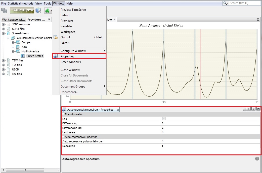
Auto-regressive spectrum’s properties

1. The spectral graphs are available from: Tools → Spectral analysis.

   

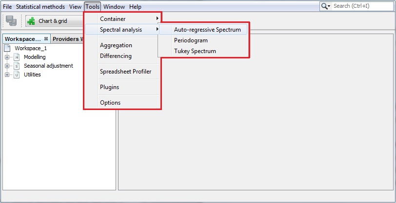
   Tools for spectral analysis

2. When the first option is chosen JDemetra+ displays an empty Auto-regressive spectrum window. To start an analysis drag a single time series from the Providers window and drop it into the Drop data here area.

   

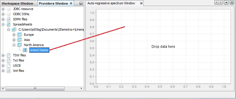
   Launching an auto-regressive spectrum

3. An auto-regressive spectrum graph available in JDemetra+ is based on the relevant tool from the X-13ARIMA-SEATS program. It shows the spectral density (spectrum) function, which reformulates the content of the stationary time series’ autocovariances in terms of amplitudes at frequencies of half a cycle per month or less. The number of observations, data transformations and other options such as the specification of the frequency grid and the order of the autoregressive polynomial (30 by default) can be specified by opening the Window → Properties from the main menu.

   The Auto-regressive - Properties window contains the following options:

   • Log - a log transformation of a time series;

   • Differencing - transforms a data by calculating a regular (order 1,2..) or seasonal (order 4, 12, depending on the time series frequency) differences;

   • Differencing lag - the number of lags that the program will use to take differences. For example, if Differencing lag = 3 then the differencing filter does not apply to the first lag (default) but to the third lag.

   • Last years - a number of years at the end of the time series taken to produce autoregresive spectrum. By default, it is 0, which means that the whole time series is considered.

   • Auto-regressive polynomial order - the number of lags in the AR model that is used to estimate the spectral density. By default, the order of the autoregressive polynomial is set to 30 lags.

   • Resolution - the value 1 plots the spectral density estimate for the frequencies $\omega_{j} = \frac{2\pi j}{n}$, where $n \in ( - \pi;\pi)$ is the size of the sample used to estimate the AR model. Increasing this value, which is set to 5 by default, will increase the precision of this grid.

4. The seasonality test described above uses an empirical criterion to check whether the series has a seasonal component that is predictable (stable) enough that it can be estimated with reasonable success. The peak in the auto-regressive spectrum has to be greater than the median of the 61 spectrum ordinates and has to exceed the two adjacent spectral values by more than a critical value. When such a case is detected, the test results are displayed in green.

   

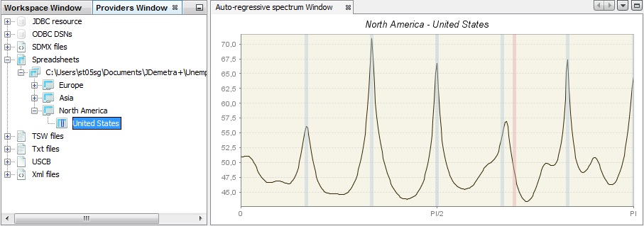
   An example of an-auto-regressive spectrum

5. The second spectral graph is a periodogram. To perform the analysis of a single time series using this tool, choose Tools →Spectral analysis → Periodogram and drag and drop a series from the Providers window to the empty Periodogram window.

   

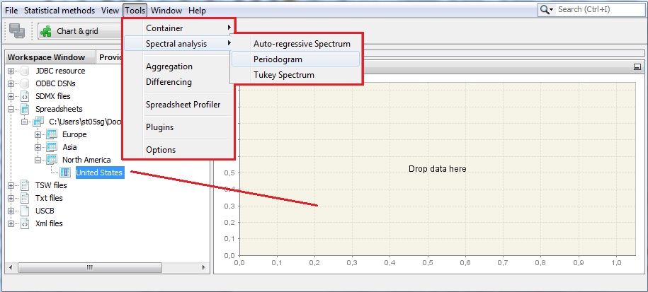
   Launching a periodogram

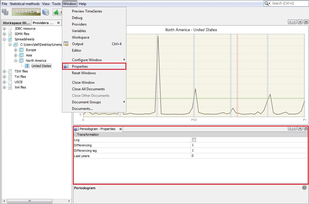
6. The sample size and data transformations can be specified by opening the Window → Properties, in the main menu. The Periodogram - Properties window contains the following options:

   • Log - a log transformation of a time series;

   • Differencing - transforms the data by calculating regular (order 1,2..) or seasonal (order 4, 12, depending on the time series frequency) differences;

   • Differencing lag - the number of lags that you will use to take differences. For example, if Differencing lag = 3 then the differencing filter does not apply to the first lag (default) but to the third lag.

   • Last years - the number of years at the end of the time series taken to produce periodogram. By default it is 0, which means that the whole time series is considered.

   

   Periodogram’s properties

7. The periodogram was one of the earliest tools used for the analysis of time series in the frequency domain. It enables the user to identify the dominant periods (or frequencies) of a time series. In general, the periodogram is a wildly fluctuating estimate of the spectrum with a high variance and is less stable than an auto-regressive spectrum.

   

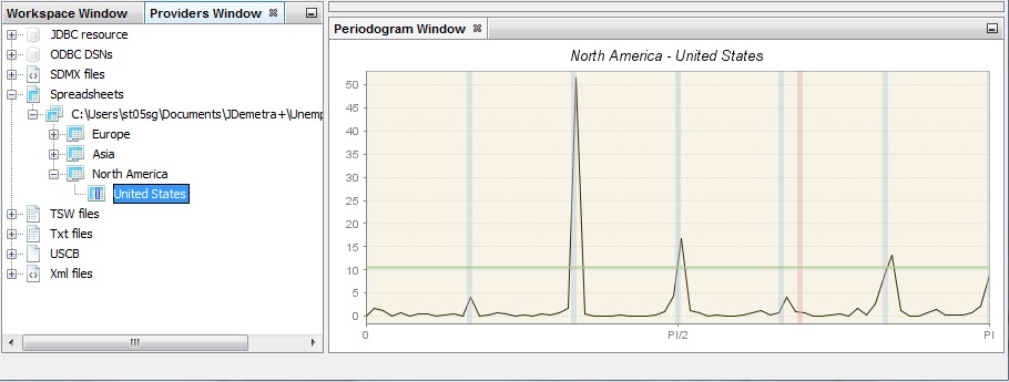
   An example of a periodogram

8. The third spectral graph is the Tukey spectrum. To perform the analysis of time series using this tool, choose Tools → Spectral analysis → Tukey spectrum and drag and drop a single series from the Providers window to the empty Periodogram window.

   

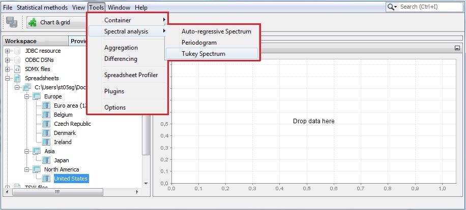
   Launching a Tukey spectrum

9. The Tukey spectrum estimates the spectral density by smoothing the periodogram.

   

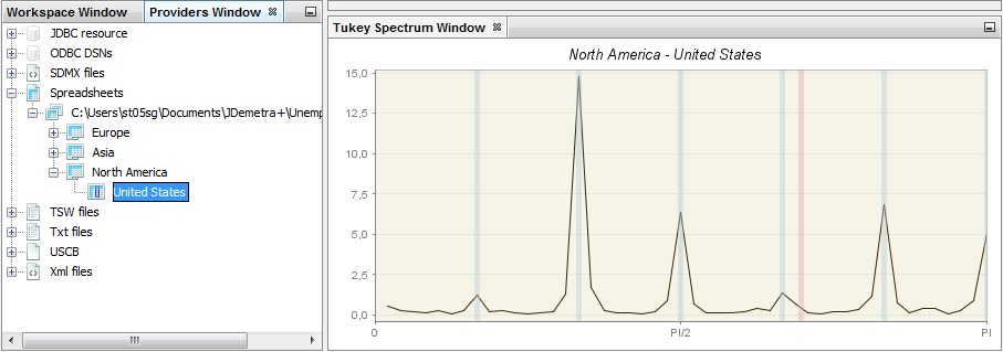
   An example of a Tukey spectrum

10. The options for the Tuckey window can be specified by opening the Window → Properties from the main menu. The Periodogram - Properties window contains the following options:

    • Log - a log transformation of a time series.

    • Differencing - transforms the data by calculating regular (order 1, 2..) or seasonal (order 4, 12, depending on the time series frequency) differences.

    • Differencing lag - the number of lags that you will use to take differences. For example, if Differencing lag = 3 then the differencing filter does not apply to the first lag (default) but to the third lag.

    • Taper part – parameter larger than 0 and smaller or equal to one that shapes the curvature of the smoothing function that is applied to the auto-covariance function.

    • Window length – the size of the window that is used to smooth the auto-covariance function. A value of zero includes the whole series.

    • Window type – it refers to the weighting scheme that it is used to smooth the auto-covariance function. The available windows types (Square, Welch, Tukey, Barlett, Hamming, Parzen) are suitable to estimate the spectral density.

    

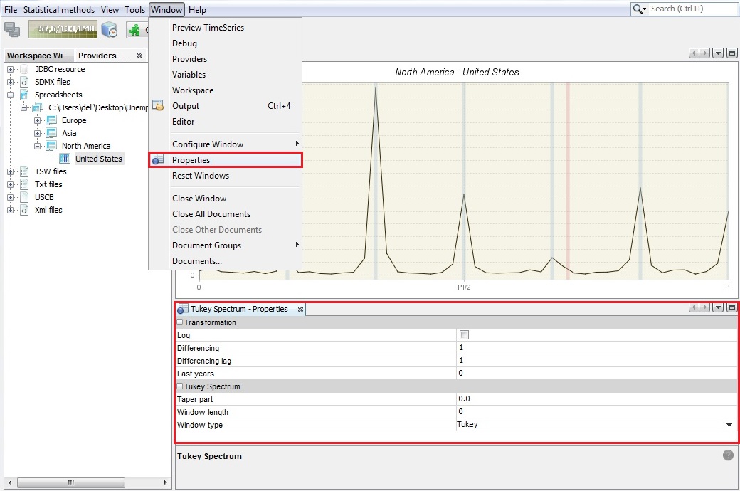
    Tukey spectrum’s properties