User-defined outliers

Outliers¹ are abnormal values of a time series. In general, they cannot be properly explained by the ARIMA model and its underlying normality assumption. They tend to be associated with irregular special events that produce a distortion in the series. The presence of such values disturbs the modelling of time series with methods like X-13ARIMA-SEATS and TRAMO-SEATS because of the linear procedures (e.g. moving averages and regression analysis) implemented by them. The presence of outliers has an adverse effect on the quality of seasonal adjustment because outliers can lead to model misspecification, biased parameter estimation, poor forecasts and inappropriate decomposition of a series. Therefore, it is vital to identify and include them in the modelling step of seasonal adjustment. The aim is to remove the effect of outliers from a time series before its decomposition into its components. Both X-13ARIMA-SEATS and TRAMO-SEATS include automatic procedure for the treatment of outliers (detection and correction). However, a priori information about an event that may have caused the abnormal observations (the date of its occurrence and type of an effect) can be included in the model by the user. This case study explains how to do it.

In the automatic outlier detection and correction procedures, three outlier types are considered by default:

• additive outlier (AO) – an abnormal value in an isolated point of the series;

• transitory change (TC) – a series of outliers with a temporarily decreasing effect on the level of the series;

• level shift (LS) – series of innovation outliers with a constant long-term effect on the level of the series, where for an innovation outlier is meant an anomalous value in the innovation series.

Seasonal outliers, which are defined as an abrupt increase or decrease of the seasonal component for a specific month or quarter and are of permanent nature can be automatically detected once the user has chosen the appropriate option. The relevant instructions are given in this case study.

The user may also introduce into the model a ramp effect, which is described as a smooth, linear transition between two time points unlike the abrupt change associated with level shifts. This case study explains how to add ramp effects into a specification.

The formulas that describe outliers are given here.

1. The picture below presents the number of registered unemployed persons in Poland. It is clear that in the beginning of 1999 a sudden, permanent shift in the trend level took place as a result of the poor state of the economy. At the end of 2008 a single peak can be observed, which can be interpreted as a reaction by entrepreneurs to the beginning of the economic crisis.

   

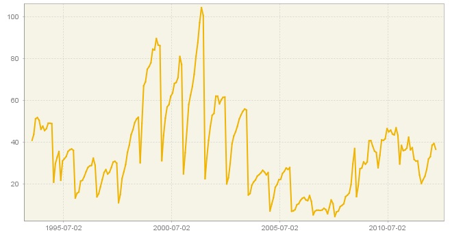
   Registered unemployed persons in Poland

2. To include these events in the model, first create and open a new specification.

3. In the Regression section choose the Pre-defined outliers item.

   

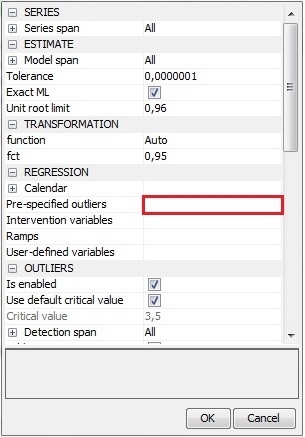
   Activating the Pre-specified outliers option

4. In a newly opened window choose the start date of the outlier (here: 01.1999) and its type. Note that more than one outlier can be assigned to the specific time period.

   

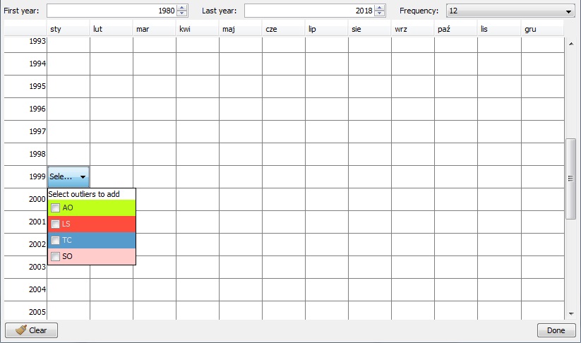
   An input window for entering a pre-specified outlier

5. Enter the relevant information for the next outlier and when all pre-defined outliers are entered, click Done.

   

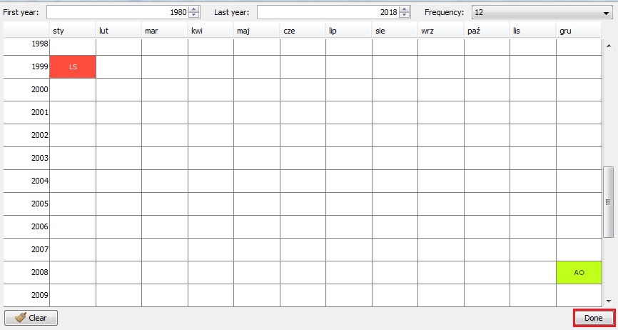
   Confirming the settings for the pre-specified outliers

6. Pre-specified outliers are visible in the Specification window. The start date and type of user-defined outliers are not verified in the seasonal adjustment process. Click OK to confirm your choice.

   

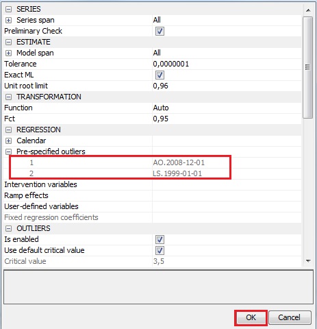
   Specification that includes the pre-specified outliers

7. Use the newly created specification to perform the seasonal adjustment using a Multi Processing option (see Simple seasonal adjustment of a single time series scenario.

   

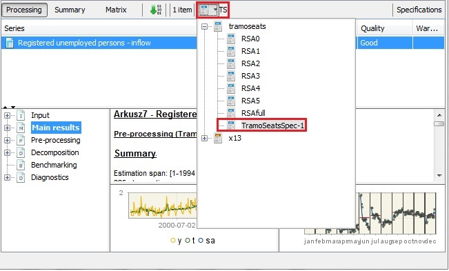
   Choosing a specification

8. Go to the pre-processing node and analyse the output. The outliers are divided into two parts: pre-specified outliers introduced by the user and outliers identified by the software.

   

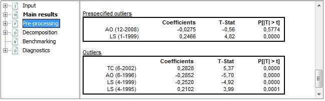
   Summary statistics for the pre-specified outliers

9. If some changes are needed (e.g. in the analysed example the pre-specified outlier AO (12-2008) is not statistically significant) click on the Specification button and modify the settings in the Pre-specified outliers section.

   

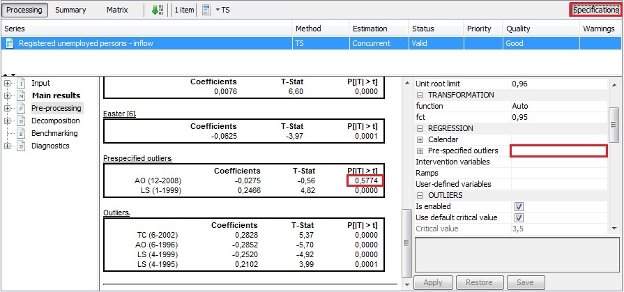
   Modifying a specification

10. Automatic identification of the seasonal outliers is performed once the user marks the seasonal outlier item in the Specification window and confirms this choice with the Apply button. Detected seasonal outliers (if any) are displayed in the pre-processing panel.

    

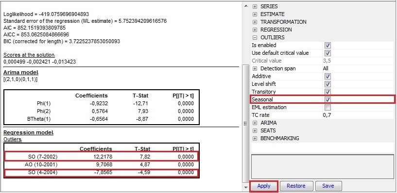
    Launching the automatic identification of seasonal outliers

11. Alternatively, the user may include the identification and estimation of seasonal outliers in the user-defined specification by marking the Seasonal option in the Outliers section.

12. To include a Ramp effect go to the Regression part of the specification and click the Ramp effects item.

    

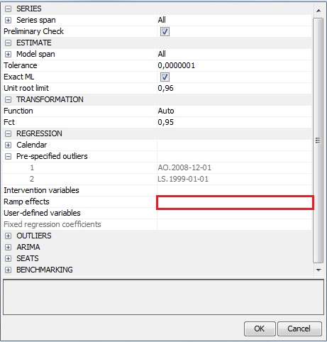
    Activating a ramp option

13. In a newly opened window use “+” button to add the ramp effect. Modify the start and end date of the effect. Add more ramps if necessary and click Done.

    

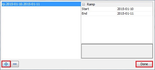
    Introducing the parameters for a ramp regression variable

14. Ramps are visible in the Regression section. Click Apply to confirm your input and analyse the output.

    

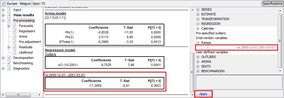
    Estimation results for a ramp regression variable