Simple seasonal adjustment of a single time series

This scenario guides the user through all the steps of the process required to seasonally adjust a single time series. Links to the appropriate parts of the Reference Manual for detailed explanations are provided when necessary.

1. Go to the main menu and follow the path: Statistical methods → Seasonal adjustment → Single analysis. Select a seasonal adjustment method (TramoSeats (i.e. the TRAMO-SEATS method will be used) or X13 (i.e. the X13ARIMA-SEATS will be used).

   

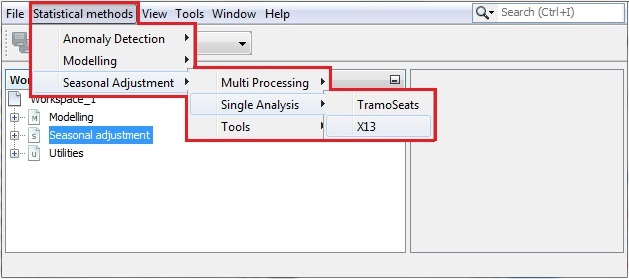
   Launching seasonal adjustment for a single time series

2. An empty panel will be opened. The picture below shows the view when the X-13ARIMA-SEATS method is chosen.

   

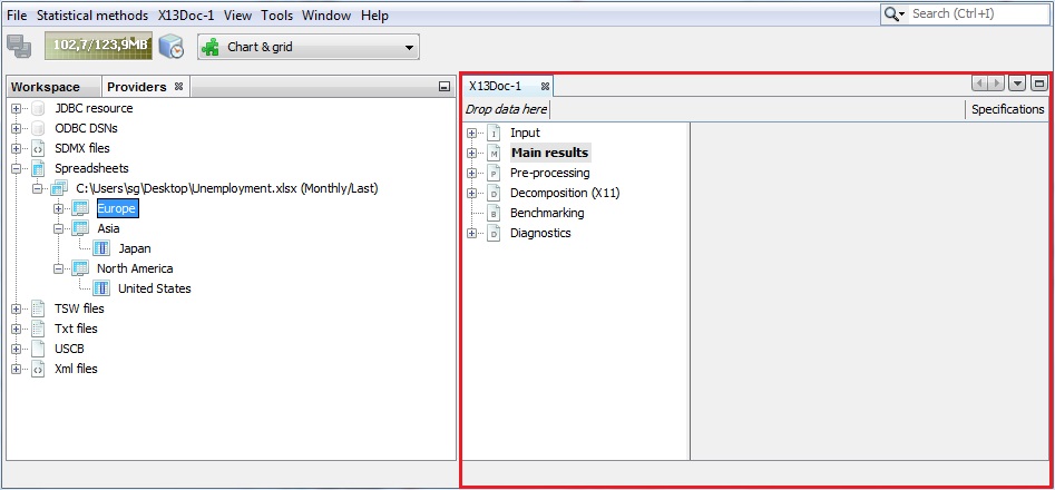
   Single analysis window

3. Select a data provider and unfold an already imported dataset. Drag and drop one time series from the Providers window to the Drop data here box as shown below. The window contains two panels. The one on the left presents the structure of the output in the form of an output tree. The other one is empty. Once the seasonal adjustment has been performed, this panel will show detailed results for any item chosen by the user from the output tree.

   

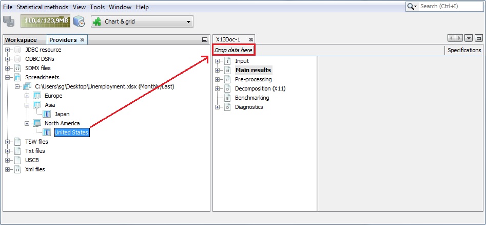
   Starting a seasonal adjustment process

4. When the user drops a series into the document window (X13Doc in the example presented in this scenario) JDemetra+ starts the seasonal adjustment process automatically. By default, a summary of results is displayed. It is accompanied by two graphs: an overlay graph on the left with the original unadjusted series, the seasonally-adjusted series and the trend-cycle and the SI ratio graph on the right. The diagnostics and graphs for the modelling part are discussed here. The user can find also find some explanations of the results of seasonal adjustment for X-13ARIMA-SEATS and for TRAMO-SEATS). The Main results panel provides a quick summary of the quality of the adjustment. Study the diagnostics section using the vertical scrollbar.

   

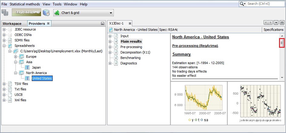
   Simple seasonal adjustment, single time series: main results panel

5. The results are highlighted in green, yellow or red, depending on the result of the statistical test used. Green indicates that problematic characteristics have not been detected (e.g. lack of normality of residuals, autocorrelation in residuals). Yellow indicates that the test outcome is uncertain. Those in red indicate that there are issues that should be addressed. The user is expected to investigate the problematic test statistics and try to improve the model, so that no uncertain or rejected test results are present.

   

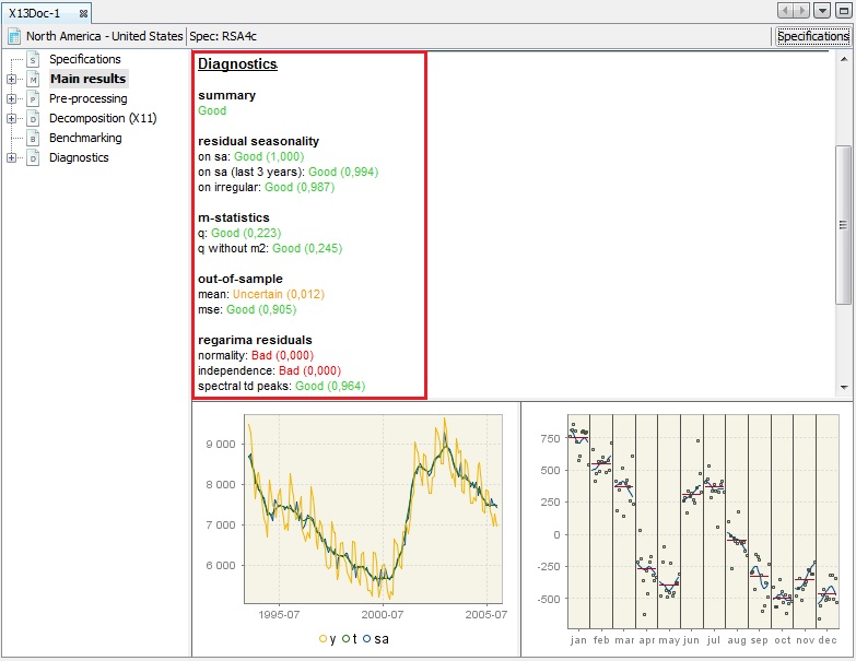
   Diagnostic results - simple seasonal adjustment of single time series

6. To explore the results, expand the tree in the left panel and click on the desired node. Here Out-of-sample test was chosen.

   

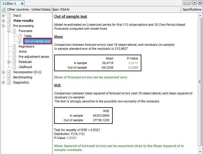
   Exploring the results

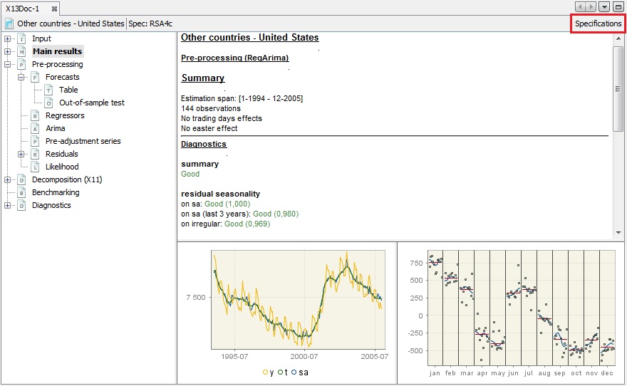
7. The default specification used for a seasonal adjustment can be modified by clicking on the Specifications button.

   

   Changing a default specification

8. The Specifications panel presents settings that have been used to generate the current output.

   

   Specification panel

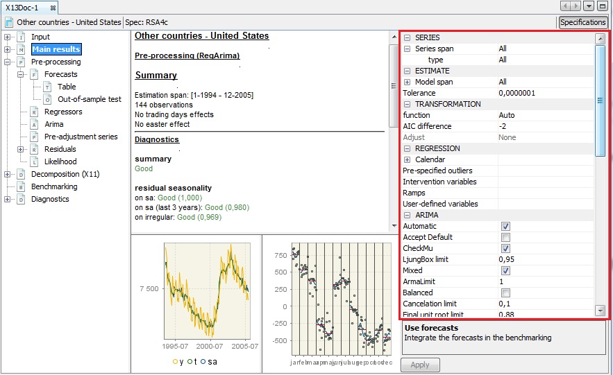
9. To change a given setting, click on it and choose an option from the list and/or enter a value. In the picture below the series span was shortened by the first 12 observations. Inputs in green indicate that the entered values are acceptable (appropriate format, data within the allowed range and so on). To apply the changes click on the Apply button in the bottom part of the window.

   

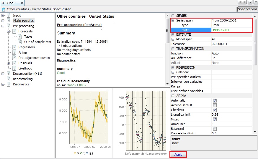
   Modifying settings

10. Be aware that the changes introduced may lead to changes in the output for other parts of the results. The example below illustrates that omitting the first 12 observations results in automatic detection of trading day effects and the Easter effect, which were not present in the previous model.

    

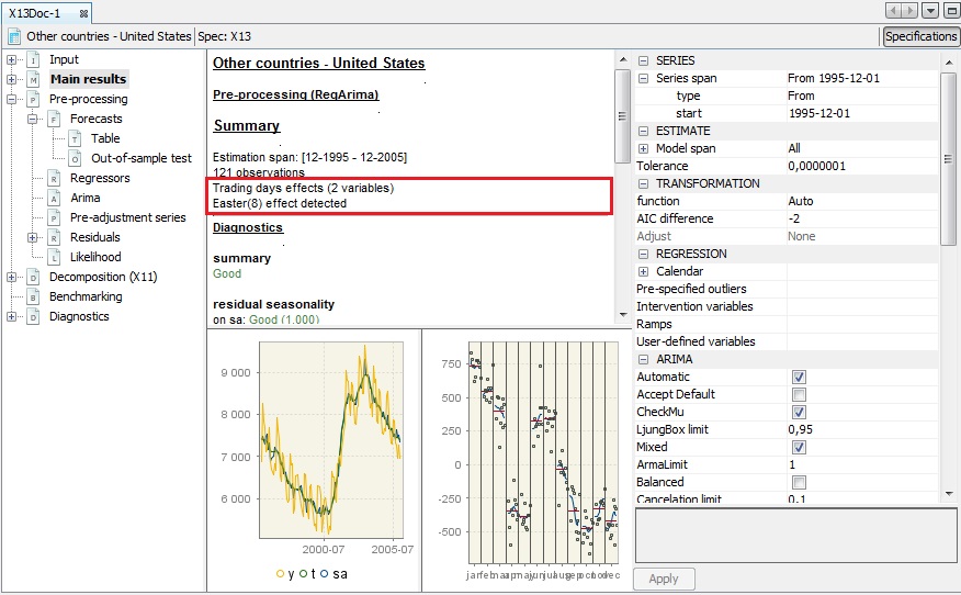
    The effect of applying modified settings

11. To copy the estimated series (seasonally adjusted, trend, seasonal and irregular) to another file go to the Table item in the Main results section of the output tree. Then click on the upper-left cell in the table.

    

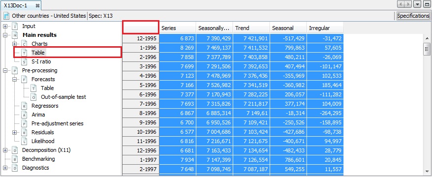
    Highlighting the output series

12. Copy the series by clicking the Copy item from the context menu or use the standard Ctrl+C keys. Other options from this menu are explained here.

    

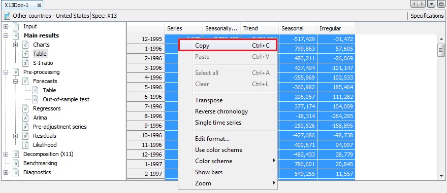
    Copying the series

13. Paste the series to the destination file (e.g. TXT, Excel).

    

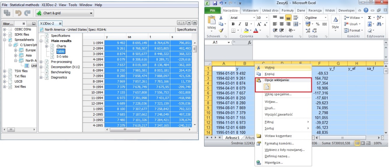
    Easy exporting data to an Excel file

14. To save the document created in JDemetra+ (named X13Doc-1 in our example) select Save Workspace As… item from the File menu.

    

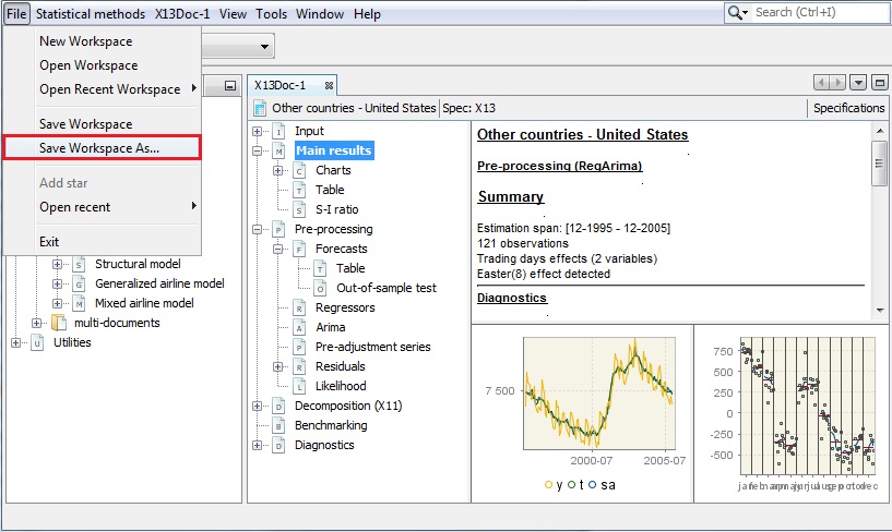
    Saving a workspace

15. Enter the location, workspace name and click Save.

    

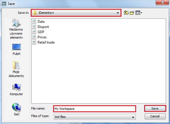
    Choosing a destination folder

16. The document is visible in the Workspace window under the appropriate section (x13 in the case presented in the picture). The document can be opened, deleted or renamed from the context menu.

    

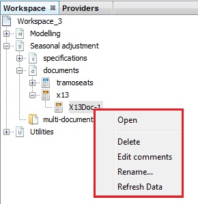
    The content of the context menu for a single document

17. The user can also add comments to the document. To display the comments and modify them, click on Edit comments from the context menu.

    

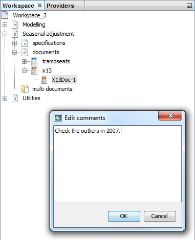
    An example of an Edit comments window

18. At the end of this process, the user is presented with the results already saved in the workspace. The option Refresh data becomes active when the given workspace is opened again. This option can be activated either from a local menu or from the main menu. Once it is activated, JDemetra+ refers to the data source defined in the workspace and uses this current version of data to perform seasonal adjustment with the settings saved in the document.

    

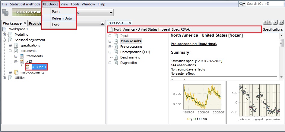
    Refreshing the data