Direct versus indirect approach

Economic time series are often computed and reported according to a certain classification or a breakdown. For example, in National Accounts total consumption expenditures are a sum of individual consumption expenditures and General Government & NPISHs consumption expenditures. Therefore, the seasonally adjusted aggregates can be computed either by aggregating the seasonally adjusted components (indirect adjustment) or adjusting the aggregate and the components independently (direct adjustment). The point is that these two strategies result in different seasonally adjusted aggregates. As neither theoretical nor empirical evidence uniformly favours one approach over the other, the choice of the seasonal adjustment strategy concerning aggregated series depends on the user¹. Guidance in this field is given in the ESS Guidelines on Seasonal Adjustment (2015)

1. JDemetra+ offers a Direct–Indirect Seasonal Adjustment functionality that facilitates the comparison of the results from these two strategies, which is launched from the main menu.

   

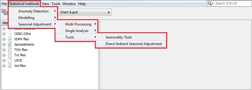
   The Direct-Indirect Seasonal Adjustment tool

2. To start the analysis drag and drop time series to the top-left panel. The panel on the right presents the sum of selected series.

   

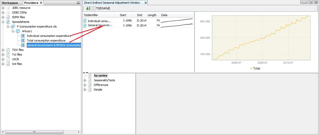
   Choosing series for an analysis

3. By going to the main menu and clicking on Window → Properties, one can specify benchmarking options for direct-indirect comparison. Be aware that the properties window displays the properties of an active item. Therefore, first click on the time series graph in the picture below and then activate the Properties window.

   

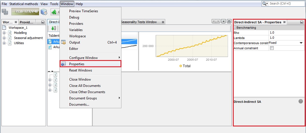
   The properties of the Direct - Indirect seasonal adjustment functionality

4. By default, the pre-defined TRAMO-SEATS specification is used (RSAfull) for seasonal adjustment of a dataset. To change it, click on the button marked in the picture below. This will provide you with the alternative specifications. Here the user defined specification named My spec is chosen.

   

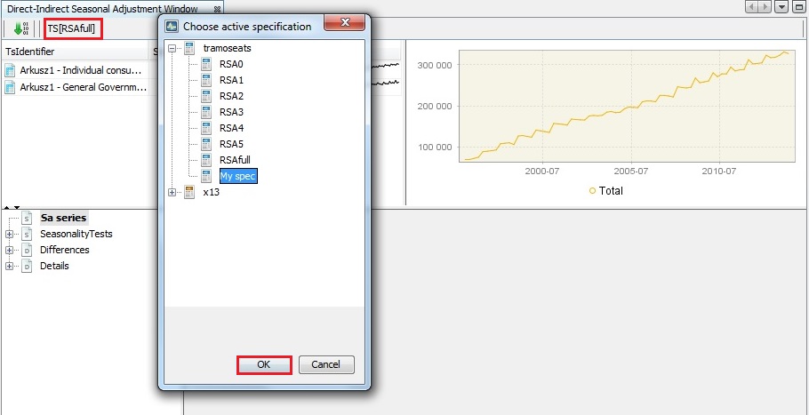
   Choosing a specification for the analysis

5. Next, run the process by clicking the button with the green arrow.

   

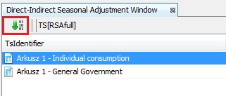
   Running a process

6. The bottom panel presents the detailed results. The seasonality test node presents the outcome of the seasonality tests performed for the aggregated series adjusted directly (Direct sa) and indirectly (Indirect sa). The reason for presenting these tests here is that the presence of residual seasonality and calendar effects should be monitored, especially in the indirectly adjusted series². It might happen that the seasonality is successfully removed from the components but it is still present in the aggregated series.

   

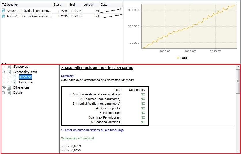
   Seasonality tests’ results for a direct seasonal adjustment

7. The Differences node presents selected different results between the direct and the indirect seasonal adjustment approaches. The Statistics section shows basic statistics (average, standard deviation, minimum and maximum) for the relative differences (%) between the direct and the indirect SA series. Chart contains the graph of the differences, while Table includes the actual values. The Periodogram section presents graphs for two spectral estimators – the periodogram and the auto-regressive spectrum.

   

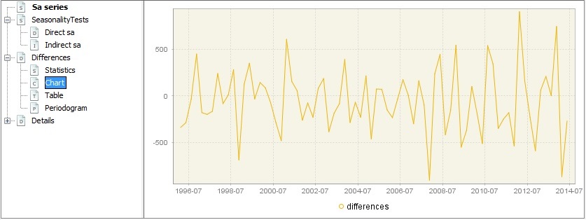
   Graph presenting the differences between direct and indirect seasonal adjustment results

8. The Details node include the basic statistics for the relative differences between the benchmarked and original series as well as the actual time series adjusted directly (Sa series) and indirectly (Benchmarked Sa series).

   

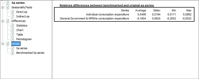
   Details of the differences between direct and indirect seasonal adjustment results