Identification of seasonal peaks in autoregressive spectrum
AR Spectrum definition
The estimator of the spectral density at frequency \(\lambda \in [0,\pi]\) will be given by the assumption that the series will follow an AR(p) process with large \(p\). The spectral density of such model, with an innovation variance \(var(x_{t})=\sigma^2_x\), is expressed as follows:
\[10\times log_{10} f_x(\lambda)=10\times log_{10} \frac{\sigma^2_x}{2\pi \left|\phi(e^{i\lambda}) \right|^2 }=10\times log_{10} \frac{\sigma^2_x}{2\pi \left|1-\sum_{k=1}^{p}\phi_k e^{i k \lambda}) \right|^2 }\]where \(\phi_k\) denotes the AR(k) coefficient, and \(e^{-ik\lambda}=cos(-ik\lambda)+i sin(-ik\lambda)\).
Soukup and Findely (1999) suggest the use of p=30, which in practice much larger than the order that would result from the AIC criterion. The minimum number of observations needed to compute the spectrum is set to n=80 for monthly data (or n=60) for quarterly series. In turn, the maximum number of observations considered for the estimation is n=121. This choice offers enough resolution, being able to identify a maximum of 30 peaks in a plot of 61 frequencies: by choosing \(\lambda_j=\pi j/60\),for \(j=0,1,…,60\), we are able to calculate our density estimates at exact seasonal frequencies (1, 2, 3, 4, 5 and 6 cycles per year). Note that \(x\) cycles per year can be converted into cycles per month by simply dividing by twelve, \(x/12\), and to radians by applying the transformation \(2\pi(x/12)\).
The traditional trading day frequency corresponding to 0.348 cycles per month is used in place of the closest frequency \(\pi j/60\). Thus, we replace \(\pi 42/60\) by \(\lambda_{42}=0.348\times 2 \pi = 2.1865\). The frequencies neighbouring \(\lambda_{42}\) are set to \(\lambda_{41}= 2.1865-1/60\) and \(\lambda_{43}= 2.1865+1/60\). The periodogram below illustrates the proximity of this trading day frequency \(\lambda_{42}\) (red shade) and the frequency corresponding to 4 cycles per year \(\lambda_{40}=2.0944\). This proximity is precisely what poses the identification problems: the AR spectrum boils down to a smoothed version of the periodogram and the contribution of the of the trading day frequency may be obscured by the leakage resulting from the potential seasonal peak at \(\lambda_{40}\), and vice-versa.
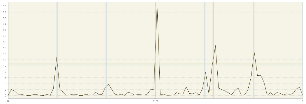
Periodogram with seasonal (grey) and calendar (red) frequencies highlighted
JDemetra+ allows the user to modify the number of lags of this estimator and to change the number of observations used to determine the AR parameters. These two options can improve the resolution of this estimator.
Graphical Test
The statistical significance of the peaks associated to a given frequency can be informally tested using a visual criterion, which has proved to perform well in simulation experiments. Visually significant peaks for a frequency \(\lambda_{j}\) satisfy both conditions:
- \(\frac{f_{x}(\lambda_{j})- \max \left\{f_{x}(\lambda_{j+1}),f_{x}(\lambda_{j-1}) \right\}}{\left[ \max_{k}f_{x}(\lambda_{k})-\min_{i}f_{x}(\lambda_{i}) \right]}\ge CV(\lambda_{j})\), where \(CV(\lambda_{j})\) can be set equal to \(6/52\) for all \(j\)
- \(f_{x}(\lambda_{j})> median_{j} \left\{ f_{x}(\lambda_{j}) \right\}\), which guarantees \(f_{x}(\lambda_{j})\) it is not a local peak.
The first condition implies that if we divide the range \(\max_{k}f_{x}(\lambda_{k})-\min_{i}f_{x}(\lambda_{i})\) in 52 parts (traditionally represented by stars) the height of each pick should be at least 6 stars.
Use
The test can be applied directly to any series by selecting the option Statistical Methods » Seasonal Adjustment » Tools » Seasonality Tests. This is an example of how results are displayed for the case of a monthly series:
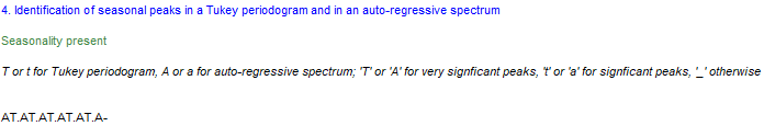
JDemetra+ considers critical values for \(\alpha=1\%\) (code “A”) and \(\alpha=5\%\) (code “a”) at each one of the seasonal frequencies represented in the table below, e.g. frequencies $\frac{\pi}{6},\ \frac{\pi}{3},\ \frac{\pi}{2},\ \frac{2\pi}{3}\text{ and } \frac{5\pi}{6}\ $ corresponding to 1, 2, 3, 4, 5 and 6 cycles per year in this example, since we are dealing with monthly data. The codes “t” and “T” correpond to the so-called Tukey spectrum, so ignore them for the moment.
The seasonal and trading day frequencies by time series frequency
| Number of months per full period | Seasonal frequency | Trading day frequency (radians) |
|---|---|---|
| 12 | $\frac{\pi}{6},\frac{\pi}{3},\ \frac{\pi}{2},\frac{2\pi}{3},\ \frac{5\pi}{6},\ \pi$ | $d$, 2.714 |
| 6 | $\frac{\pi}{3},\frac{2\pi}{3}$, $\pi$ | \(d\) |
| 4 | $\frac{\pi}{2}$, $\pi$ | $d$, 1.292, 1.850, 2.128 |
| 3 | \(\pi\) | \(d\) |
| 2 | \(\pi\) | \(d\) |
Currently, only seasonal frequencies are tested, but the program allows you to manually plot the AR spectrum and focus your attention on both seasonal and trading day frequencies. Agustin Maravall has conducted a simulation experiment to calculate \(CV(\lambda_{42})\) (trading day frequency) and proposes to set for all \(j\) equal to the critical value associated to the trading frequency, but this is currently not part of the current automatic testing procedure of JDemetra+.
References
- Soukup, R.J., and D.F. Findley (1999) On the Spectrum Diagnosis used by X12-ARIMA to Indicate the Presence of Trading Day Effects After Modeling or Adjustment. In Proceedengs of the American Statistical Association. Business and Economic Statistics Section, 144-149, Alexandria, VA.