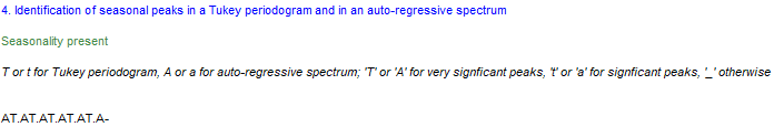
Identification of seasonal peaks in a Tukey spectrum
Tukey Spectrum definition
The Tukey spectrum belongs to the class of lag-window estimators. A lag window estimator of the spectral density \(f(\omega)=\frac{1}{2\pi}\sum_{k<-\infty}^{\infty}\gamma(k)e^{i k \omega}\) is defined as follows: \(\hat{f}_{L}(\omega)=\frac{1}{2\pi}\sum_{\left| h \right| \leq r } w(h/r)\hat{\gamma}(h)e^{i h \omega}\)
where \(\hat{\gamma}(.)\) is the sample autocovariance function, \(w(.)\) is the lag window, and \(r\) is the truncation lag. \(\left| w(x)\right|\) is always less than or equal to one, \(w(0)=1\) and \(w(x)=0\) for \(\left| x \right| > 1\). The simple idea behind this formula is to down-weight the autocovariance function for high lags where \(\hat{\gamma}(h)\) is more unreliable. This estimator requires choosing \(r\) as a function of the sample size such that \(r/n \rightarrow 0\) and \(r\rightarrow \infty\) when \(n \rightarrow \infty\) . These conditions guarantee that the estimator converges to the true density.
JDemetra+ implements the so-called Blackman-Tukey (or Tukey-Hanning) estimator, which is given by \(w(h/r)=0.5(1+cos(\pi h/r))\) if \(\left| h/r \right| \leq 1\) and \(0\) otherwise.
The choice of large truncation lags \(r\) decreases the bias, of course, but it also increases the variance of the spectral estimate and decreases the bandwidth.
JDemetra+ allows the user to modify all the parameters of this estimator, including the window function.
Graphical Test
The current JDemetra+ implementation of the seasonality test is based on a \(F(d_{1},d_{2})\) approximation that has been originally proposed by Maravall (2012) for TRAMO-SEATS. This test is has been designed for a Blackman-Tukey window based on a particular choices of the truncation lag \(r\) and sample size. Following this approach, we determine visually significant peaks for a frequency \(\omega_{j}\) when
\[\frac{2 f_{x}(\omega_{j})}{\left[ f_{x}(\omega_{j+1})+ f_{x}(\omega_{j-1}) \right]} \ge CV(\omega_{j})\]where \(CV(\omega_{j})\) is the critical value of a \(F(d_{1},d_{2})\) distribution, where the degrees of freedom are determined using simulations. For \(\omega_{j}= \pi\), we have a significant peak when \(\frac{f_{x}(\omega_{[n/2]})}{\left[ f_{x}(\omega_{[(n-1)/2]})\right]} \ge CV(\omega_{j})\)
Two significant levels for this test are considered: \(\alpha=0.05\) (code “t”) and \(\alpha=0.01\) (code “T”).
As opposed to the AR spectrum, which is computed on the basis of the last \(120\) data points, we will use here all available observations. Those critical values have been calculated given the recommended truncation lag \(r=79\) for a sample size within the interval \(n \in [80,119]\) and \(r=112\) for \(n \in [120,300]\) . The \(F\) approximation is less accurate for sample sizes larger than \(300\). For quarterly data, \(r=44\), but there are no recommendations regarding the required sample size
Use
The test can be applied directly to any series by selecting the option Statistical Methods » Seasonal Adjustment » Tools » Seasonality Tests. This is an example of how results are displayed for the case of a monthly series:
JDemetra+ considers critical values for \(\alpha=1\%\) (code “T”) and \(\alpha=5\%\) (code “t”) at each one of the seasonal frequencies represented in the table below, e.g. frequencies $\frac{\pi}{6},\ \frac{\pi}{3},\ \frac{\pi}{2},\ \frac{2\pi}{3}\text{ and } \frac{5\pi}{6}\ $ corresponding to 1, 2, 3, 4, 5 and 6 cycles per year in this example, since we are dealing with monthly data. The codes “a” and “A” correpond to the so-called AR spectrum, so ignore them for the moment.
The seasonal and trading day frequencies by time series frequency
| Number of months per full period | Seasonal frequency | Trading day frequency (radians) |
|---|---|---|
| 12 | $\frac{\pi}{6},\frac{\pi}{3},\ \frac{\pi}{2},\frac{2\pi}{3},\ \frac{5\pi}{6},\ \pi$ | $d$, 2.714 |
| 6 | $\frac{\pi}{3},\frac{2\pi}{3}$, $\pi$ | \(d\) |
| 4 | $\frac{\pi}{2}$, $\pi$ | $d$, 1.292, 1.850, 2.128 |
| 3 | \(\pi\) | \(d\) |
| 2 | \(\pi\) | \(d\) |
Currently, only seasonal frequencies are tested, but the program allows you to manually plot the Tukey spectrum and focus your attention on both seasonal and trading day frequencies.
References
- Tukey, J. (1949). The sampling theory of power spectrum estimates., Proceedings Symposium on Applications of Autocorrelation Analysis to Physical Problems, NAVEXOS-P-735, Office of Naval Research, Washington, 47-69