Inflation forecasting using the R package rjssf
by David De Antonio Liedo
Here, I will describe the main features of the model developed
by Basselier, de Antonio Liedo, Jonckehere and Langenus (2018), and illustrate
how it can be estimated using the R package rjssf, which exploits the Java libraries defining the state-space
framework (SSF) of JDemetra+. A completely unrelated SSF application regarding the specification of an error
component structure to improve signal extraction in surveys can be
found here.
A multivariate model with trend and cycles that simultaneously appear in multiple equations
The first two equations represent inflation and unemployment, which are typically analyzed together in order to understand the business cycle component of inflation. The variable \(\tau^{\pi}_{t}\) represents the trend in inflation (which is common to core inflation) and it follows a random walk process. We also specify an unobserved component \(\textcolor{blue}{\delta_{t}}\), which can be interpreted as a business cycle factor that is common to most of the macroeconomic variables considered in the system. Also, \(\textcolor{magenta}{\vartheta_{t}}\) appears in the inflation equation representing the effect of energy prices. Of course this component also appears in the equation for oil prices. Here, I will not give further details on the model, but two important remarks:
- First of all, notice that we are incorporating a large number of variables to the system (to the best of my knowledge, much larger than any other model of the same class published in the literature). The information set includes import prices \(\pi^{m}_{t}\), oil prices in logs \(P^{oil}_{t}\), real GDP \(y_{t}\) a business survey \(S^{Y}_{t}\) and an estimate of the yearly growth in markups \(\mu_{t}\) \(\begin{eqnarray} \pi_{t} &=& \kappa_{\pi}\tau^{\pi}_{t} + \lambda_{\pi} \textcolor{blue}{\delta_{t}} + \zeta_{\pi} \textcolor{magenta}{\vartheta_{t}} + \eta^{\pi}_{t} \\ u_{t} &=& \tau^{u}_{t} + \kappa_u \textcolor{blue}{\delta_{t}} + \eta^{u}_{t} \\ \pi^{core}_{t} &=& \tau^{\pi}_{t} + \lambda_{core} \textcolor{cyan}{\delta_{t-4}} + \eta^{core}_{t} \\ \pi^{m}_{t} &=& \tau^{m}_{t} + \zeta_{m} \textcolor{magenta}{\vartheta_{t}} + \eta^{M}_{t} \\ P^{oil}_{t} &=& \tau^{oil}_{t} + \zeta_{oil}\textcolor{magenta}{\vartheta_{t}} + \eta^{oil}_{t} \\ y_{t} &=& \tau^{y}_{t} + \kappa_y \textcolor{blue}{\delta_{t}} + \eta^{y}_{t} \\ S^{Y}_{t} &=& m_{S} + \kappa_{S} (\textcolor{blue}{\delta_{t}} -\textcolor{cyan}{\delta_{t-4}})+ \eta^{S}_{t} \\ \mu_{t} &=& m_{\mu} + \kappa_{\mu} (\textcolor{blue}{\delta_{t}} -\textcolor{cyan}{\delta_{t-4}})+ \eta^{\mu}_{t} \end{eqnarray}\)
-
The model incorporates additional variables that represent inflation expectations, and they are introduced in a model-consistent way. As an example of observables to which \(\pi^{E}_{t}\) refers we have qualitative survey data (e.g. Business and Consumer expectations), quantitative data (e.g. ECB Survey of Professional Forecasters), or financial variables (e.g. interest rates). \(\begin{eqnarray} \underbrace{\pi^{E}_{t} }_{E[\pi_{t+h}|t]} &=& \tau^{\pi}_{\textcolor{red}{t+h|t}} + \lambda_{\pi} \delta_{\textcolor{red}{t+h|t}} + \zeta_{\pi} \vartheta_{\textcolor{red}{t+h|t}} + \eta^{\pi}_{\textcolor{red}{t+h|t}} \end{eqnarray}\)
-
Notice that the subindex \(\textcolor{red}{t+h|t}\) represents the expected value of the components at time \(t+h\) conditional on the information set available upto \(t\). The expression for the expectations of the trend components are straightforwards, as it will be shown below (for the measurement errors, the expected values are zero unless we relax the I.I.D. assumption). However, the expectations for the components \(\textcolor{blue}{\delta_{t}}\) or \(\textcolor{magenta}{\vartheta_{t}}\) will be a linear combination of their current value and their first lag, since we will assume they follow a stationary AR(2) process. Since the resulting coefficients may be non-linear combinations of the autoregresive dynamics, we prefer to incorporate the expectational terms explicitely in the state-space representation of the AR(2) model (notice the state vector incorporates both forecasts and lagged values). This representation is more complicated than the one typically used for an AR(2) model opens in new tab, and this has implications for the way in which we will define the measurement equations.
-
The trend \(\tau^{\pi}_t\) is common to inflation and core inflation, and it follows a random walk without drift, which correspond to a particular parameterization of the local level model (opens in a new tab). The same model is used for \(\tau^{m}_t\). The trend in the log of oil prices, \(\tau^{oil}_t\), is assumed to be a random walk with drift, which we specify it as a restricted version of the local linear trend model (opens in a new tab) with both level and slope variances equal to zero. Both \(\tau^{y}_t\) and \(\tau^{u}_t\) are assumed to be smooth trends, which are also versions of the local linear trend model (opens in a new tab) with level variance equal to zero. No trend is required in the stationary variables, but a constant term or intercept is added ( \(m_S\) and \(m_{\mu}\)). In this case, we simply define it as local level model (opens in a new tab) with null variance.
- The \(\eta\) terms refer to measurement errors, which we will specify as I.I.D. Below, we will explain how to specify them.
Specifying the model in R
Here, we will specify a slightly more complicated model than the one depicted above. Our aim is to decompose inflation into the following three components:
- Trend
- Business cycle effect
- Energy prices component
- Non-energy related component of imports
The last component implies we need to define an additional common component in the equations for the import deflator, total and core inflation.
DEFINING THE STOCHASTIC PROCESS FOR THE TRENDS AND OTHER COMPONENTS
The first step is to define the latent variables (=unobserved components) and determine a stochastic process for each of them.
# Define the model
modelX<-jd3_ssf_model()

# create the trend components and add them to the model
add(modelX, jd3_ssf_locallineartrend("tu", levelVariance = 0, fixedLevelVariance = TRUE ))
add(modelX, jd3_ssf_locallineartrend("ty", levelVariance = 0, fixedLevelVariance = TRUE)) #
add(modelX, jd3_ssf_locallevel("tpi"))
add(modelX, jd3_ssf_locallevel("intcore", variance = 0, fixed = TRUE)) # = constant for core inflation
add(modelX, jd3_ssf_locallevel("tm"))
# the trend model is t(t)=t(t-1) + z(t) + e(t), where z(t)=z(t-1)+u(t), so var(u)=0, so zt becomes the drift
add(modelX, jd3_ssf_locallineartrend("toil",slopevariance = 0, fixedSlopeVariance=TRUE,levelVariance = 0, fixedLevelVariance = TRUE))
# create the AR cycles and add them to the model: business cycle, oil prices cycle and "non-energy" imported inflation cycle
add(modelX, jd3_ssf_ar2("cycle", c(1, -.5), fixedar = FALSE, variance= 1,fixedvariance=TRUE, nlags= 4,nfcasts = 4))  # initialization c(1, -.5), variance fixed to 1
add(modelX, jd3_ssf_ar2("oilCycle", c(1, -.5), fixedar = FALSE, variance= 1,fixedvariance=TRUE, nlags= 2,nfcasts = 4))  # initialization c(1, -.5), variance fixed to 1
add(modelX, jd3_ssf_ar2("mCycle", c(1, -.5), fixedar = FALSE, variance= 1,fixedvariance=TRUE, nlags= 2,nfcasts = 4))  # initialization c(1, -.5), variance fixed to 1
# create and add measurement errors
add(modelX, jd3_ssf_ar("noiseB", c(.5), fixedar = FALSE, variance= 1,fixedvariance=TRUE, nlags= 2))  # initialization c(1, -.5), variance fixed to 1
add(modelX, jd3_ssf_ar2("noiseC", c(.5), fixedar = FALSE, variance= 1,fixedvariance=TRUE, nlags= 2,nfcasts=4))  # initialization c(1, -.5), variance fixed to 1
# create various intercepts
add(modelX, jd3_ssf_locallevel("intA", variance = 0, fixed = TRUE)) # = constant for business activity survey
add(modelX, jd3_ssf_locallevel("intB", variance = 0, fixed = TRUE)) # = constant for inflation business survey
add(modelX, jd3_ssf_locallevel("intC", variance = 0, fixed = TRUE)) # = constant for inflation consumer survey
# intercepts for markup
add(modelX, jd3_ssf_locallevel("int_mu", variance = 0, fixed = TRUE))
MEASUREMENT EQUATIONS
In order to define the measurement equations for the system, we would need to know the exact order of the various components within the state
vector and the composition of each component block. Luckily, we will only need to know how each block has been defined and there will be no need
to input the correct paraeters in the system matrices. The program will do it for you, as long as you specify correctly which element of each component block
you want to load on each equation. The comments in the code provide the necessary insights, but it is important to keep in mind that the block of states that contain
expectations have a very particular stucture, and the first element typically corresponds to the
lag nlag ( e.g. AR(p) model with number of lags=nlags and h forecasts )
# create the measurement equations

  eq1<-jd3_ssf_equation("eq1",variance=1, fixed = FALSE) # measurement eq for first variable (U)
  add(eq1, "tu")                                         # 1*trend + coef*cycle ; FALSE means coef is estimated  (otherwise, it is 1)

  add(eq1, "cycle", .1, FALSE, jd3_ssf_loading(4))       # nlags=4 => [y(t-4) y(t-3) y(t-2) y(t-1) y(t)]

                                                         #             0        1      2      3     4

  add(modelX, eq1)

  #---------------------------------------------------------------------------------------------------------------

  eq2<-jd3_ssf_equation("eq2",variance=1, fixed = FALSE) # measurement eq for second variable (Y)

  add(eq2, "ty")                                         # 1*trend + coef*cycle ; FALSE means coef is estimated

  add(eq2, "cycle", .1, FALSE, jd3_ssf_loading(4))

  add(modelX, eq2)

  #---------------------------------------------------------------------------------------------------------------

  eq3<-jd3_ssf_equation("eq3",variance=1, fixed = FALSE)  # measurement eq for third variable ( pi)

  add(eq3, "tpi",1, FALSE)                                # 1*trend + coef*cycle(t-p), (p=0 by default)

  add(eq3, "cycle", .5, FALSE, jd3_ssf_loading(4))        # nlags=2, h=4 => t-2, t-1 t  t+1|t  t+2|t  t+3|t  t+4|t   "2" is t and "1" is t-1 and "0" is t-p (p=2)

  add(eq3, "oilCycle", .5, FALSE, jd3_ssf_loading(2))     #                  0    1  2   3     4       5     6

  add(eq3, "mCycle", .5, FALSE, jd3_ssf_loading(2))       #                  0    1  2   3     4       5     6

  add(modelX, eq3)

  #---------------------------------------------------------------------------------------------------------------

  eq4<-jd3_ssf_equation("eq4",variance=1, fixed = TRUE)# Note in this case fixed=TRUE (we fix one variance to one because we will use the concentrated likelihood, so there will be a factor sigma multiplying all variances; if we dont do it, the program will do it, but he may choose another variable)

  add(eq4, "tpi")                                      # 1*trend + coef*cycle(t-p), p=4 in this case

  add(eq4, "cycle", .5, FALSE, jd3_ssf_loading(0))

  add(eq4, "intcore")

  add(eq4, "mCycle", .5, FALSE, jd3_ssf_loading(2))    # if the data is not normalized, a constant is needed because core is lower than total on average

  add(modelX, eq4)


  #---------------------------------------------------------------------------------------------------------------

  eq5<-jd3_ssf_equation("eq5",variance=1, fixed = FALSE)# measurement eq for fifth variable ( import price inflation)

  add(eq5, "tm")                                        # 1*trend + coef*cycle(t)

  add(eq5, "oilCycle", .5, FALSE, jd3_ssf_loading(2))   #  coefficient associated to the growth in the cycle of oil

  add(eq5, "mCycle", .5, FALSE, jd3_ssf_loading(2))

  add(modelX, eq5)


  #---------------------------------------------------------------------------------------------------------------

  eq6<-jd3_ssf_equation("eq6",variance=1, fixed = FALSE)  # measurement eq for sixth variable ( oil price)

  add(eq6, "toil")                                        # 1*trend + coef*cycle

  add(eq6, "oilCycle", .5, FALSE, jd3_ssf_loading(2))     #  coefficient associated to the growth in the cycle of oil (actually the part of the cycle that is orthogonal to the buisness cycle)

  add(modelX, eq6)


  #---------------------------------------------------------------------------------------------------------------


  eq7<-jd3_ssf_equation("eq7",variance=1, fixed = FALSE) # measurement eq for seventh variable ( markup YoY growth)

  add(eq7, "int_mu")

  add(eq7, "cycle", .1, FALSE,jd3_ssf_loading(c(4,3,2,1,0), c(1,0,0,0,-1)))

  add(modelX, eq7)

  #---------------------------------------------------------------------------------------------------------------


  eq8<-jd3_ssf_equation("eq8",variance=1, fixed = FALSE)             # measurement eq for eighth variable (Business survey: Real Activity, assuming high correlation with YoY GDP growth, cite our paper Nowcasting....Basselier et al. 2017)

  add(eq8, "intA")

  add(eq8, "cycle", .1, FALSE, jd3_ssf_loading(c(4,3,2,1,0), c(1,0,0,0,-1))) #  coefficient associated to the YoY growth in the cycle

  add(modelX, eq8)

  #---------------------------------------------------------------------------------------------------------------
Given that we want to link the consumer survey for inflation with the determinants of inflation expectations one year ahead (i.e. cummulative sum of quarterly inflation over a one year period), we will have to consider the cummulative sum of the components \(\delta_{\textcolor{red}{t+1|t}}+\delta_{\textcolor{red}{t+2|t}}+\delta_{\textcolor{red}{t+3|t}}+\delta_{\textcolor{red}{t+4|t}}\). But defining this equation correctly requires to understand the order in which the components appear in the state-space representation of the ( AR(p) model ). The definition of the business survey for inflation is simpler because we will link it to determinants of inflation one quarter ahead, e.g. \(\delta_{\textcolor{red}{t+1|t}}, \vartheta_{\textcolor{red}{t+1|t}}\), etc…
  eq9<-jd3_ssf_equation("eq9",variance=0, fixed = TRUE)      # measurement eq for Business Inflation  survey

  add(eq9, "intB")

  #add(eq9, "tpi", 1, FALSE)

  add(eq9, "cycle", .1, FALSE,jd3_ssf_loading(5))

  add(eq9, "oilCycle", .1, FALSE,jd3_ssf_loading(3))

  add(eq9, "mCycle", .1, FALSE,jd3_ssf_loading(3))

  add(eq9, "noiseB", .5, FALSE)

  add(modelX, eq9)


  #---------------------------------------------------------------------------------------------------------------

  eq10<-jd3_ssf_equation("eq10",variance=0, fixed = TRUE)       # measurement eq for Consumer

  add(eq10, "intC")

  #add(eq10, "tpi", 1, FALSE)

  add(eq10, "cycle", .1, FALSE,jd3_ssf_loading(c(5,6,7,8), c(1,1,1,1)))

  add(eq10, "oilCycle", .1, FALSE,jd3_ssf_loading(c(3,4,5,6), c(1,1,1,1)))

  add(eq10, "mCycle", .1, FALSE,jd3_ssf_loading(c(3,4,5,6), c(1,1,1,1)))

  add(eq10, "noiseC", .5, FALSE,jd3_ssf_loading(c(3,4,5,6), c(1,1,1,1)))

  add(modelX, eq10)
ESTIMATION
The model is estimated by maximum likelihood. Access the (draft) documentation to see how the estimation works (opens in a new tab)
rsltX_final<-estimate(modelX, smallDataset, precision=1e-29, marginal=TRUE, concentrated=TRUE)
Results
We will focus now on how the model is able to fit the total and core inflation series for the euro area. You can skip this part and go directly to see the graphs. Here, I just want to show you how to extract the resuts from the estimated model by defining the parameter names and the components, and assiging them an indicator of their position within the state vector.
# extract the vector of parameters
  pVector=result(rsltX_final, "parameters")
# Parameter vector has names
  names(pVector)=result(rsltX_final, "parameternames")
# Position of each component (with name)
  comppos=result(rsltX_final,"ssf.cmppos")
  names(comppos)=result(rsltX_final,"ssf.cmpnames")
# Order of each component (with name)
  comporder=seq(0,(length(comppos)-1))
  names(comporder)=result(rsltX_final,"ssf.cmpnames")
The following step may seem tedious, but it helps to assign a name to the factors we want to select, and that name will remain unchanged even if we modify the specification of the model and re-estimate it:
 # Defining strings corresponding to components

  # remember certain components contain forecasts: cycle has nlags=4, oilCycle, mCycle and noiseC have nlags=2
  # t-nlags, ..., t-4, t-3, t-2, t-1, t , t+1, ..., t+h

  tpi = paste(c("ssf.smoothing.cmp(", comporder["tpi"],")"), collapse = "")
  intcore = paste(c("ssf.smoothing.cmp(", comporder["intcore"],")"), collapse = "")

  # contain forecasts, so I use ssf.smoothing.array
  cycle  = paste(c("ssf.smoothing.array(", comppos["cycle"]+4,")"), collapse = "")
  oilCycle   = paste(c("ssf.smoothing.array(", comppos["oilCycle"]+2,")"), collapse = "")
  mCycle   = paste(c("ssf.smoothing.array(", comppos["mCycle"]+2,")"), collapse = "")
Now, we can define the fitted values for both core and total inflation:
core_fit   =(result(rsltX_final, intcore) + result(rsltX_final, tpi) + pVector["eq4.cycle"]*result(rsltX_final, cycleL4)+ pVector["eq4.mCycle"]*result(rsltX_final, mCycle))
pi_fit     =(                                                 pVector["eq3.tpi"]*result(rsltX_final, tpi) + pVector["eq3.cycle"]*result(rsltX_final, cycle)  + pVector["eq3.mCycle"]*result(rsltX_final, mCycle) + pVector["eq3.oilCycle"]*result(rsltX_final, oilCycle))
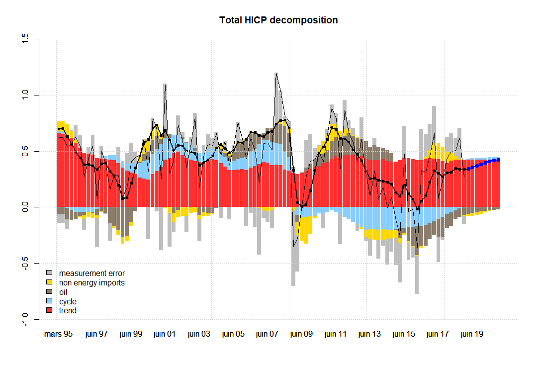
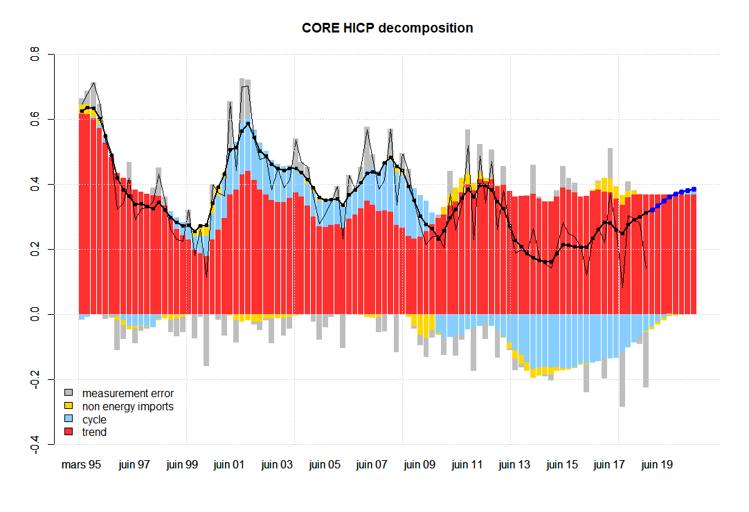
Structural decomposition and forecasting
The following graphs represent the two key variables in terms of all the unobserved components specified in the model. The thick black line with dots represents (quarterly) inflation without the measurement error given by the model. Notice that this measurement error in the case of total inflation (first graph), seems to exhibit some level of autocorrelation, while it has been specified as an IID term. In the second graph, corresponding to core inflation, we do not observe autocorrelation in the measurement error at first sight, e.g. see the grey bars, which are the difference between the thick black line with dots and the thin black line.
I decompose two of the observables (total and core inflation) into the contributions coming from all factors. The blue dots represent out-of-sample forecasts.
Understanding the sources of model misspecification is not an easy task. Some of the possible ways to improve the model without deviating from
the rjssf framework are:
- Include some lagged factors in the inflation equation (e.g. the lagged oil component)
- Add new variables to better identify the factors (e.g. more indicators related to non-energy related imports, commodities, etc…)
- Adding more indicators related to inflation expectations
- Add autocorrelation in the measurement errors (e.g. if you want to take seriously the notion that the inflation series is a bad measurement of the underlying inflation)
Ploting the unobserved components
One can also look at the unobserved components themselves. The picture below represents the smoothed value of \(\textcolor{blue}{\delta_{t}}\) conditional con the estimated parameters, and a 95$\%$ confidence interval given by the smoothed variance.
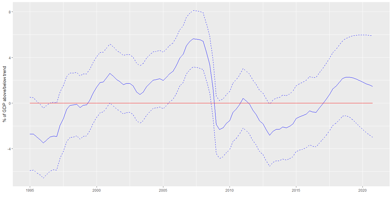
Let me show the code required to generate this graph (using ggplot)
library(ggplot2)
library(reshape2)

outputGap <- ts(result(rsltX_final, cycle)*scale, start=c(1995, 1), end=c(2020, 4), frequency=4)
outputGapL <- ts(result(rsltX_final, cycle)*scale+2*sqrt(result(rsltX_final, vCycle))*scale, start=c(1995, 1), end=c(2020, 4), frequency=4)
outputGapU <- ts(result(rsltX_final, cycle)*scale-2*sqrt(result(rsltX_final, vCycle))*scale, start=c(1995, 1), end=c(2020, 4), frequency=4)

outputGap_<-data.frame(date=time(outputGap),Y=as.matrix(outputGap) )
outputGap_L<-data.frame(date=time(outputGapL),Y=as.matrix(outputGapL) )
outputGap_U<-data.frame(date=time(outputGapU),Y=as.matrix(outputGapU) )


ggplot() +

  geom_line(data=outputGap_, aes(date, Y), color = "blue")+  geom_point() +

  geom_line(data=outputGap_L, aes(date, Y), color = "blue",linetype = "dashed" ) +

  geom_line(data=outputGap_U, aes(date, Y), color = "blue",linetype = "dashed" ) + xlab("") + ylab("Output Gap")


df <- data.frame(date=as.Date(index(outputGap)), Y = outputGap)

ggplot(outputGap)
Plotting the fitted values and decomposing it in terms of the components
Let me show you how the stacked bar decomposition has been generated. In order to obtain the plot with the decomposition, I need to define the fitted value for the components:
 # Decomposition

  core_fitCycle   =(pVector["eq4.cycle"]*result(rsltX_final, cycleL4) )

  core_fitM       =(pVector["eq4.mCycle"]*result(rsltX_final, mCycle))

  core_fitTrend   =(result(rsltX_final, intcore) +result(rsltX_final, tpi) )


  pi_fitCycle     =( pVector["eq3.cycle"]*result(rsltX_final, cycle))

  pi_fitM         =( pVector["eq3.mCycle"]*result(rsltX_final, mCycle) )

  pi_fitOil       =( pVector["eq3.oilCycle"]*result(rsltX_final, oilCycle))

  pi_fitTrend     =( pVector["eq3.tpi"]*result(rsltX_final, tpi))
I am startig to get familiar with the wonderful plotting capabilities of R, but I am not sure the function barplot does what is supposed to
do. What I did was to plot the positive contributions first and then add the negative contributions. Please let me know if you can simplify it or use a different method
# make a plot with decomposition of core inflation
# colors https://www.statmethods.net/advgraphs/parameters.html

core_fitError= core_fit*0
core_fitError[1:length(tiempo)]=-core_fit[1:length(tiempo)]+  smallDatasetFULL[,c(4)]

storeResults <- array( c( core_fitTrend, core_fitCycle, core_fitM ,core_fitError) , dim = c(length(pi_fitTrend) , 4 ) )

tiempo_f=seq(1995.25, 1995.25+(length(core_fitTrend)-1)/4, 0.25) #1980Q1to 2018Q1 (forecasts until 2020Q4)
timeDate_f=seq(as.Date("1995/3/1"), as.Date("2020/12/1"), by = "quarter")
timeDate_f=format(timeDate_f, format="%b %y")


rownames(storeResults)=tiempo_f
colnames(storeResults)=c("trend","cycle","non energy imports","measurement error")
names(core_fit)=tiempo_f


# Get the stacked barplot

myData=t(storeResults)
myData1 <- myData2 <- myData
myData1[myData1<0] <- 0  # set negative values to zero
myData2[myData2>0] <- 0  # set positive values to zero
myrange <- c(min(colSums(myData2)),max(colSums(myData1)))
mynewrange<-c(-0.4,0.8)

sampleLength=length(smallDatasetFULL[,c(4)])
fullLength=length(core_fit)

df.bar <-barplot(myData1, col=colors()[c(134,590,142,152)] , ylim=mynewrange,axisnames=TRUE,space=0.1,border = NA,beside=FALSE, names.arg=timeDate_f ,  font.axis=1)
df.bar <-barplot(myData2, col=colors()[c(134,590,142,152)] , add=TRUE,ylim=mynewrange,axisnames=TRUE,space=0.1,border = NA,beside=FALSE, names.arg=timeDate_f ,  font.axis=1,legend=colnames(storeResults),args.legend = list(x = "bottomleft", bty = "n"))
lines(x=df.bar,y=core_fit,lwd=2,col="black") %>%
points(x=df.bar,y=core_fit,lwd=2,col="black",pch=20)
lines(x=df.bar[1:sampleLength],y=smallDatasetFULL[,c(4)],lwd=1,col="black" )
lines(x=df.bar[(sampleLength+1):fullLength],y=core_fit[(sampleLength+1):fullLength],lwd=2,col="blue") %>%
points(x=df.bar[(sampleLength+1):fullLength],y=core_fit[(sampleLength+1):fullLength],lwd=2,col="blue",pch=19)
grid()
title("CORE HICP decomposition")
Posted on 12 Mar 2019
inflation forecasting structural R states space models rjssf